Fun With Frequencies

Divi Schmidt

Part 1: Gradients

In this part of the project, we examine one of the simplest but most effective kernels: the finite difference filter. This aids us in many important tasks, including edge detection and straightening.

Gradient Magnitude

For detecting edges, we calculate the magnitude of the gradient for each pixel in the image. We do this by first convolving our image with the Dx and Dy kernels. We then calculate the magnitude at each pixel using this equation.

We then determine a threshold and take all pixels with a larger magnitude as an edge pixel. Here is the result on the cameraman image.

Image after dx convolution.

Image after dy convolution.

Gradient magnitude thresholded at 0.2

In search of better edge detections, we now turn to gaussian kernels. I first created a gaussian kernel and then convolved my image with it. This gave me a blurrier image which I then calculated the gradient magnitued of. This yielded much better results as shown below.

Gradient magnitude with gaussian blur beforehand.

We can achieve the same effect by convolving a gaussian and the dx and dy kernels first, and then convolving our image with this new kernel. This works because convolutions are associative. Here are the derivative of gaussian filters that I calculated from this method.

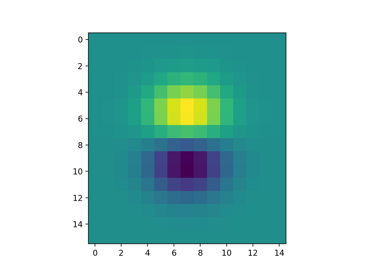
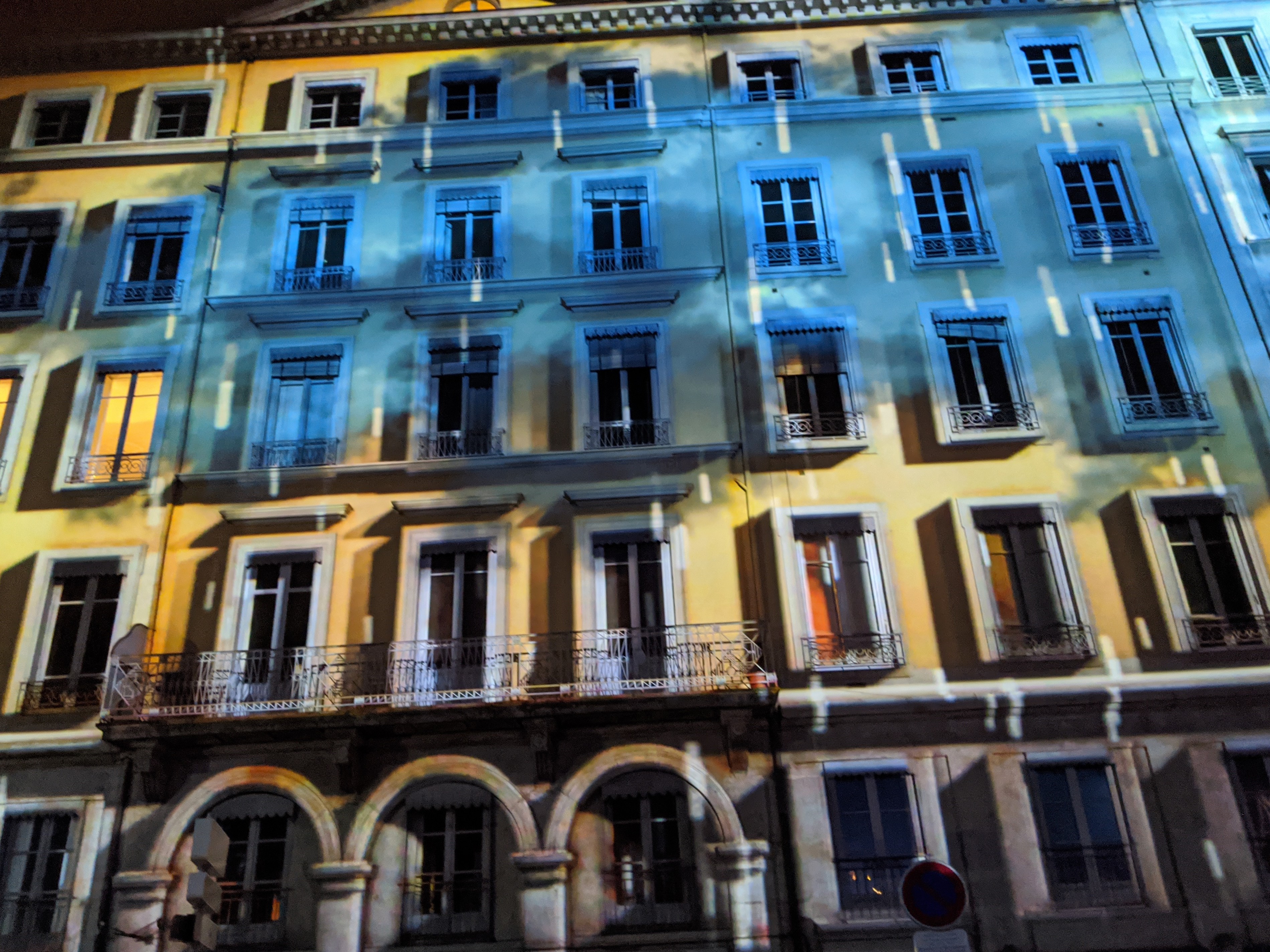
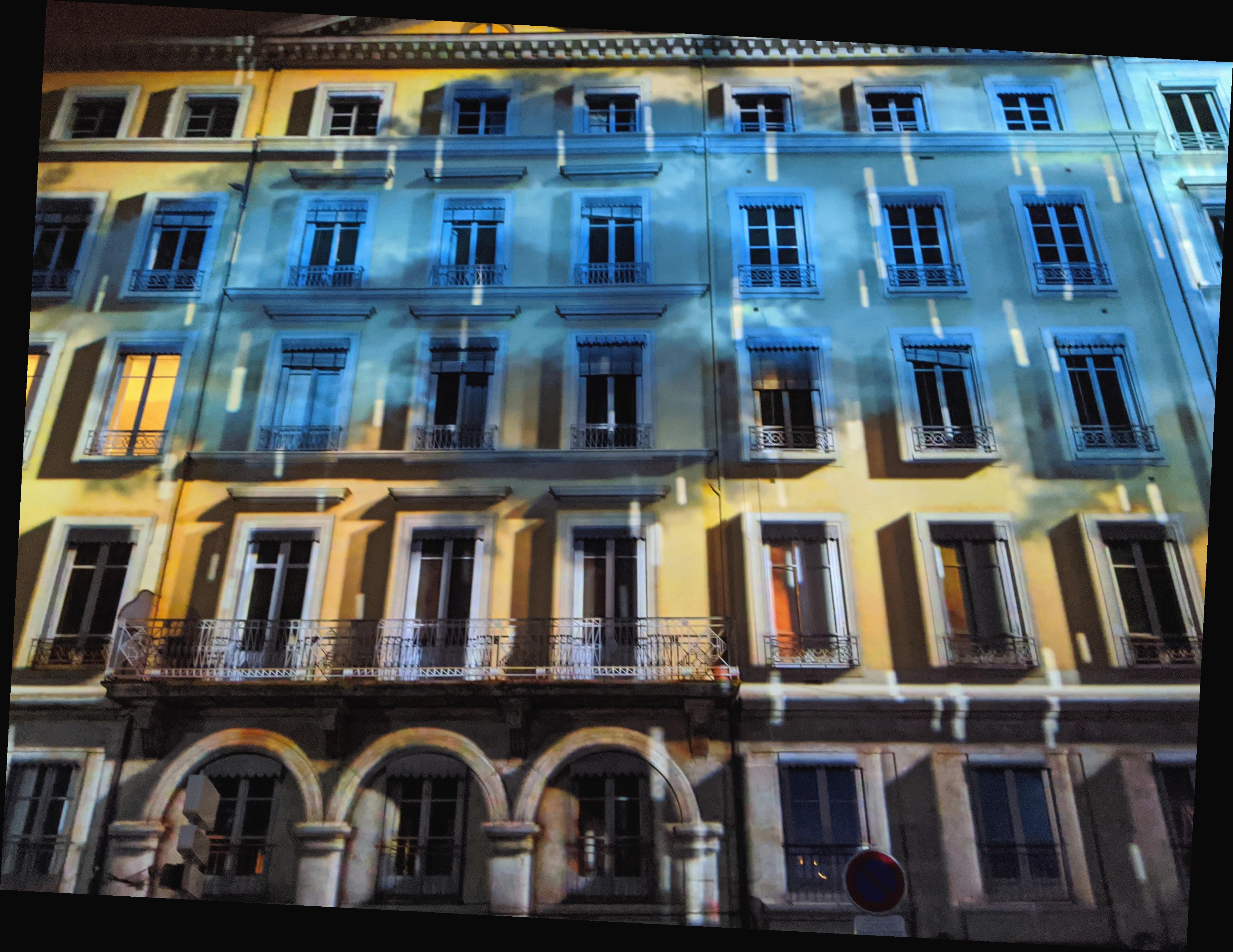
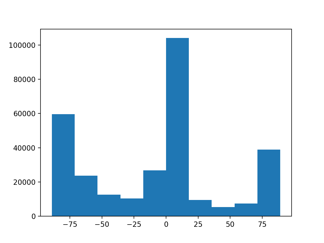
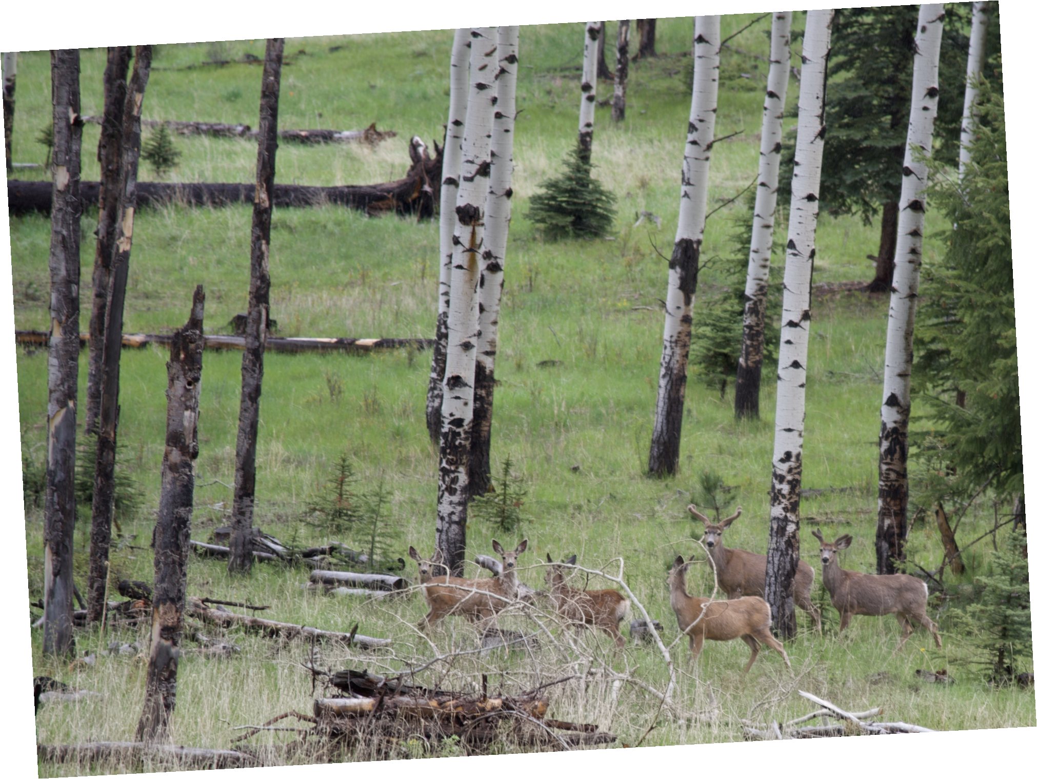
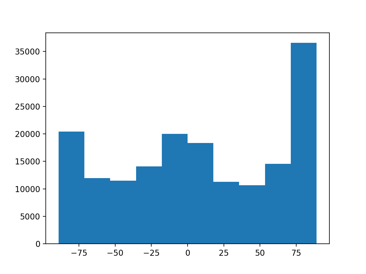
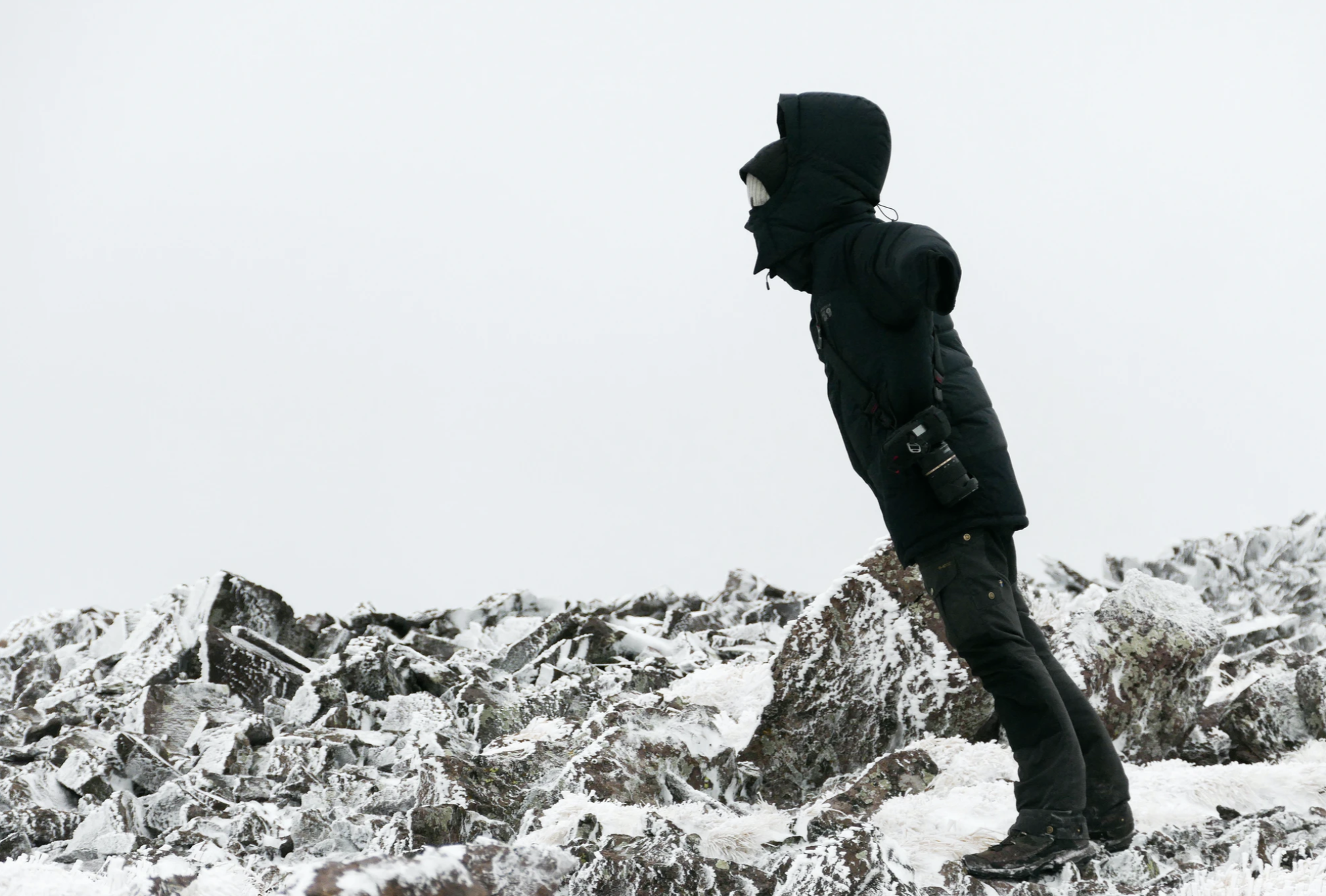
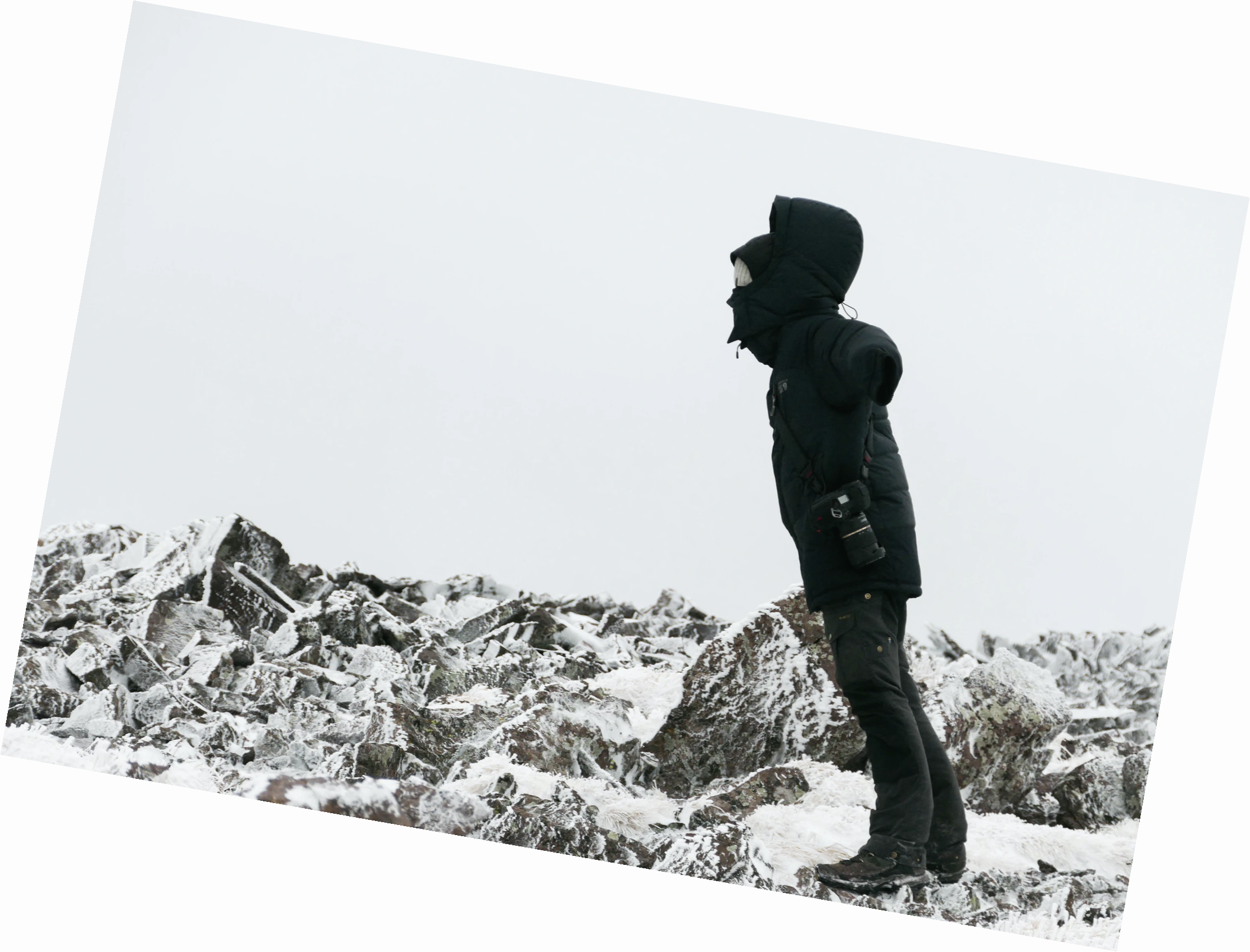
Convolution with gaussian and dx kernel.

Convolution with gaussian and dy kernel.

Image Straightening

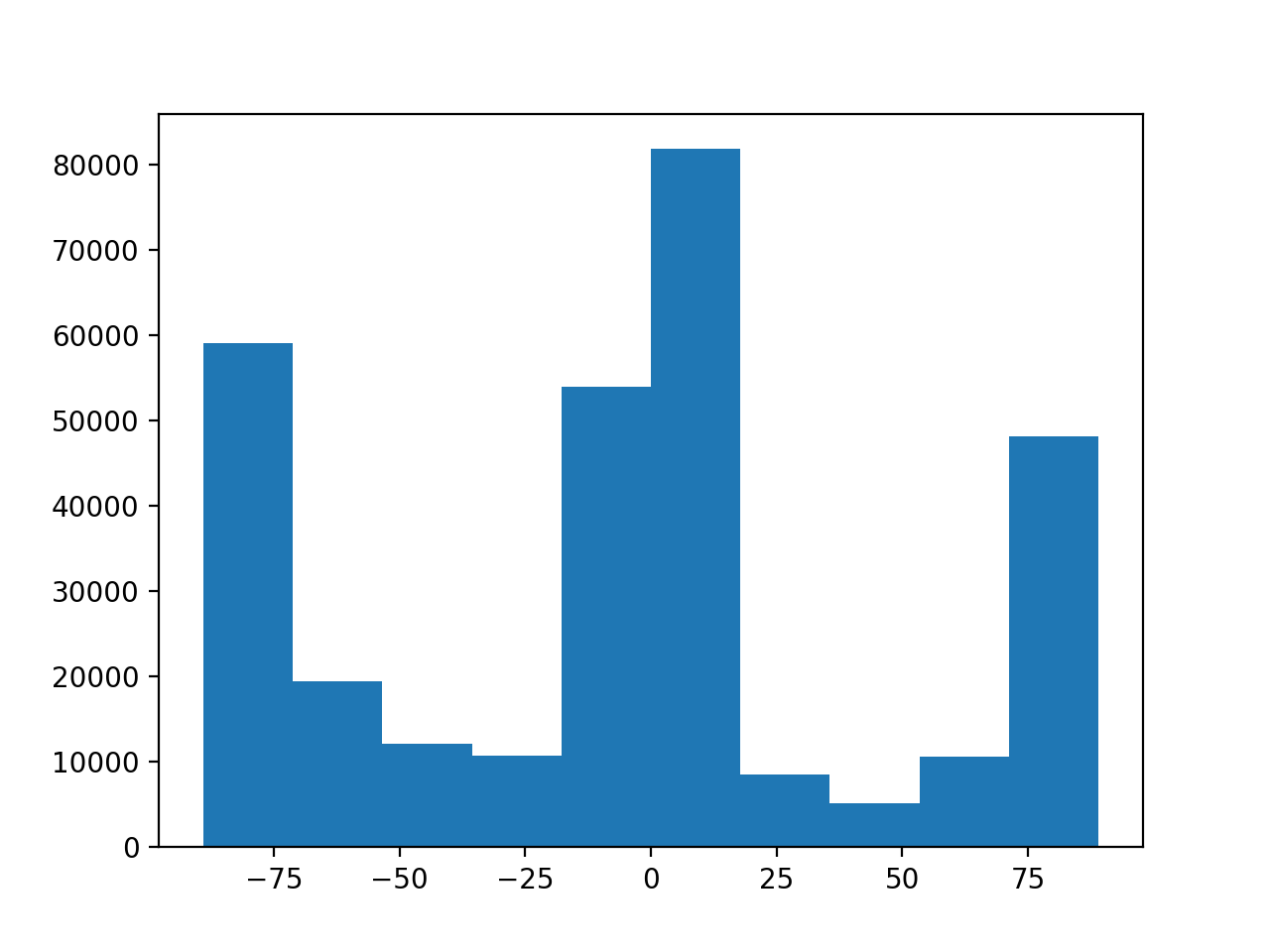
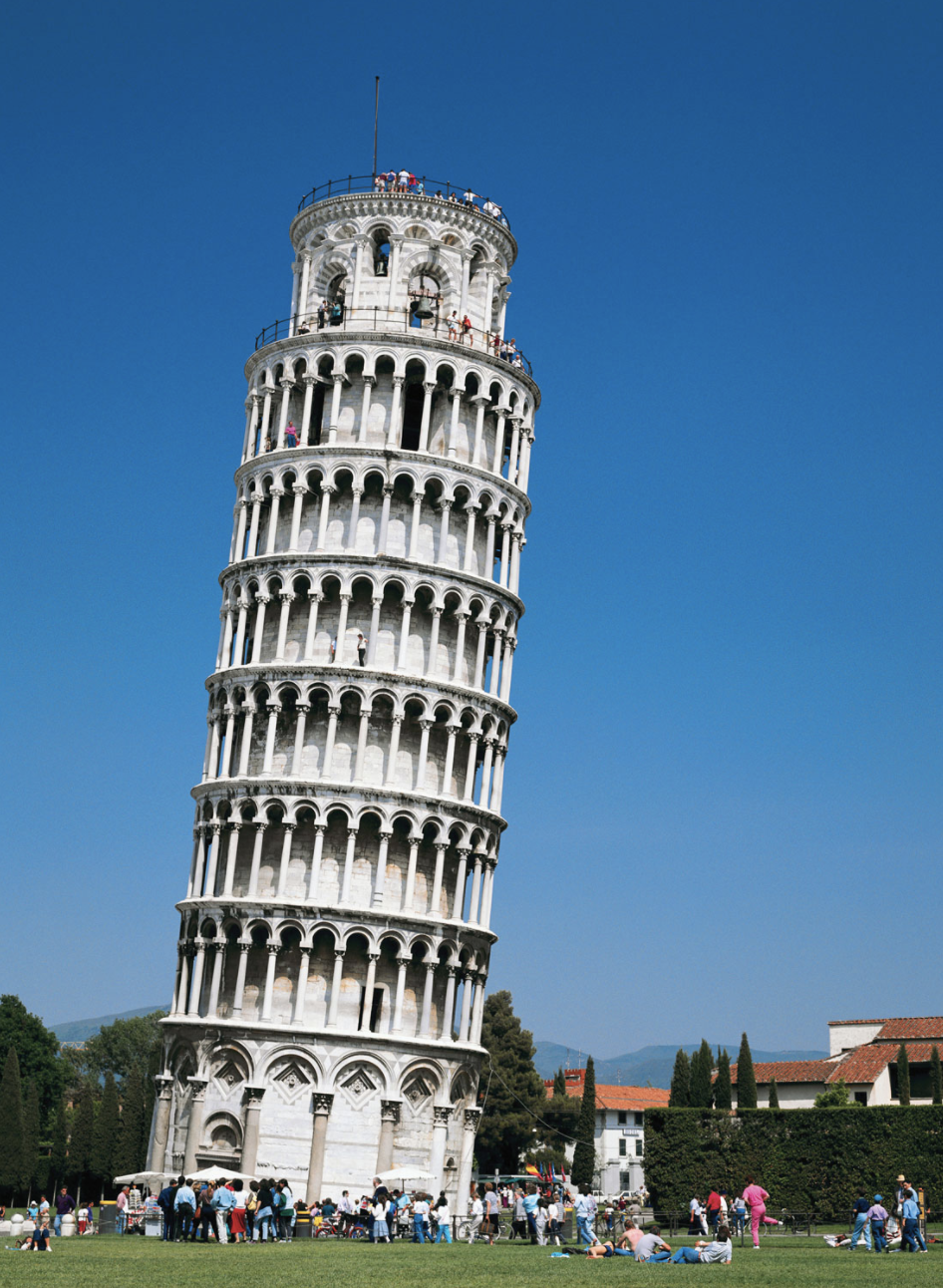
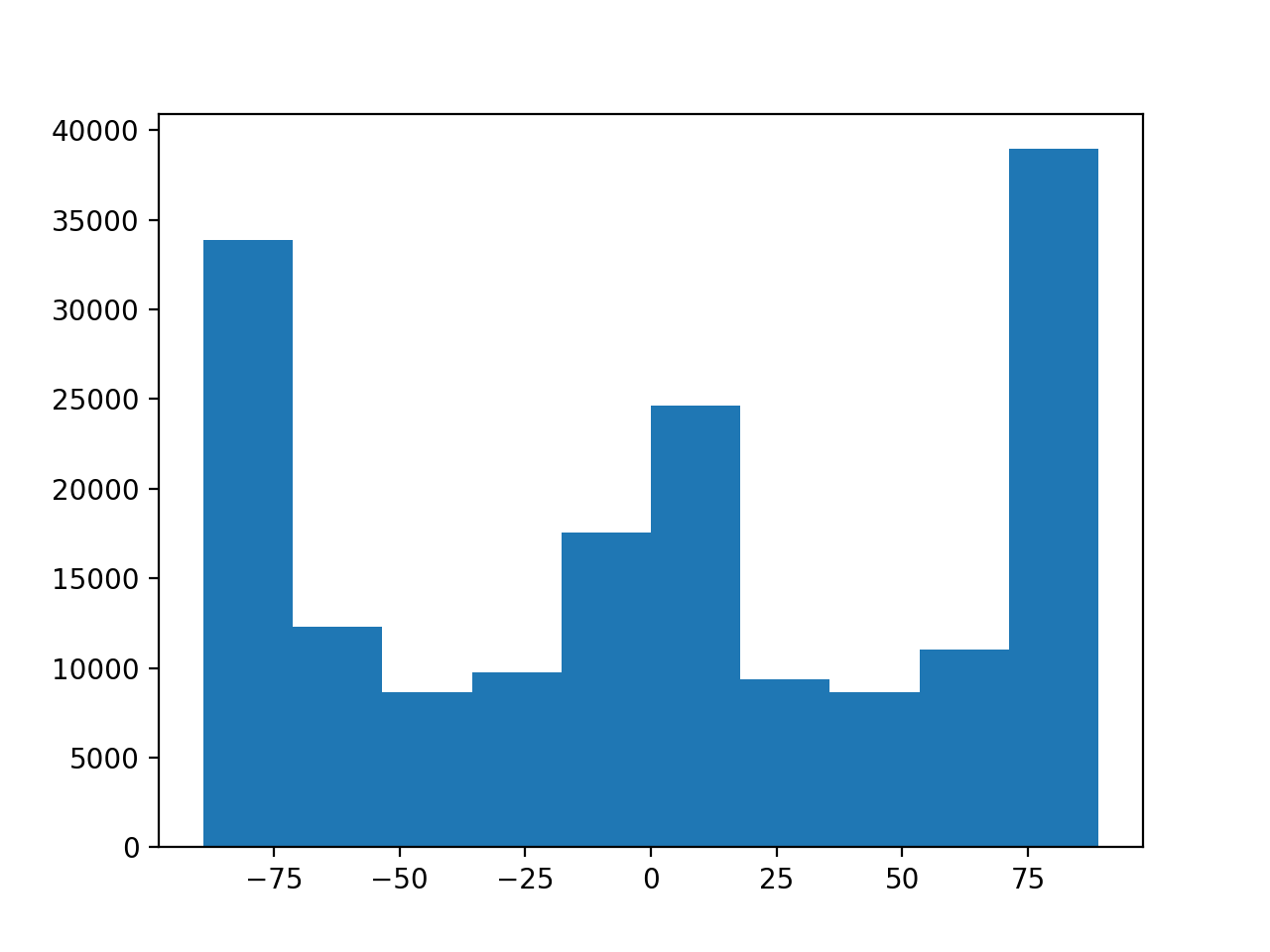
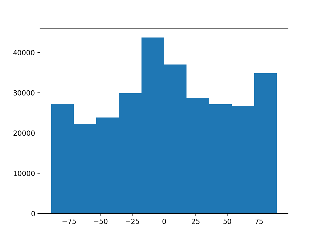
Now by using these edge detections and gradient calculations, I implemented automatic image straightening. In order to do this, I rotate an image, calculate the angle of the gradient at each pixel, and count how many angles are "good" degrees. Since we like edges to look vertical or horizontal, I counted all 90 degree 180 degree and 0 degree angles. After trying rotations within [-10, 10] degrees, I then took the rotation with the highest number of good angles. Here is the result of my straightening function on the facade image.

Original facade.	Straightened facade. Adjusted by -3 degrees.
Original facade histogram.	Straightened facade histogram.

Here are some other examples:

Leaning tower of pizza.	Straight tower of pizza.
Original pizza histogram.	Straightened pizza histogram.

Original tree image.	Straightened tree image. Adjusted by 3 degrees.
Original tree histogram.	Straightened tree histogram.

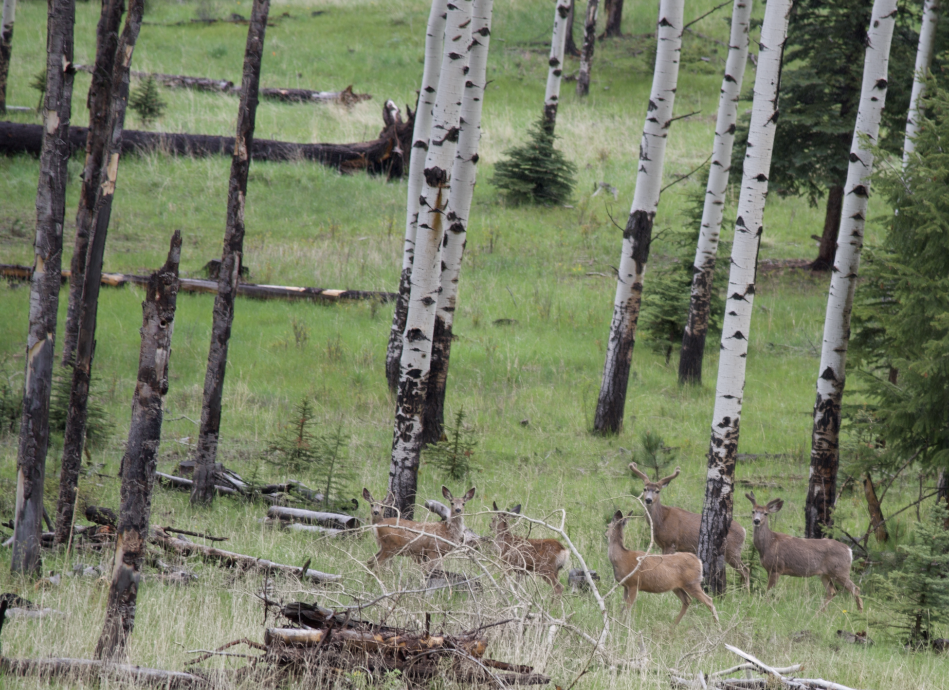
Failure case:

Original image.	Incorrectly straightened. Adjusted by -10 degrees.
Original image histogram.	"Straightened" image histogram.

Part 2

In this part of the project, we delve more into frequencies and having fun with them.

Sharpening

First, we show how increasing the higher frequencies of the image can result in a more sharp looking result. Convolving an image with a gaussian kernel will result in a low frequency image. Subtracting our original imace then gives us an image with only high frequencies. This can be added back to our original image in order to achieve the sharpening affect. This can also be done by use of the unsharp masking filter, which performs these same actions in a single convolution. Here is an example of the sharpening affect on the taj mahal.

Original image.	Sharpened with an alpha of 0.1
Sharpened with an alpha of 0.4	Sharpened with an alpha of 0.7

Now we try to sharpen an image that has been severly blurred. Notice the affect is minimal since there are not many high frequencies, and the effect that we do see is not very good.

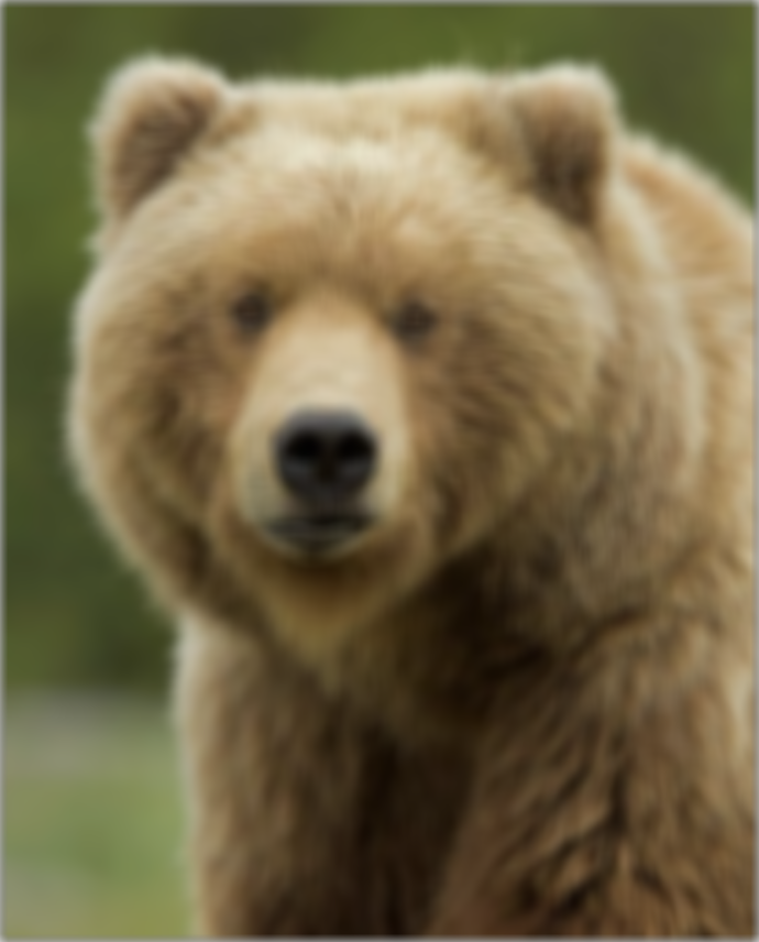
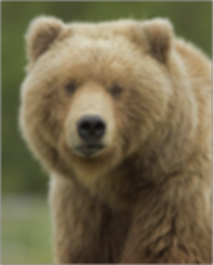
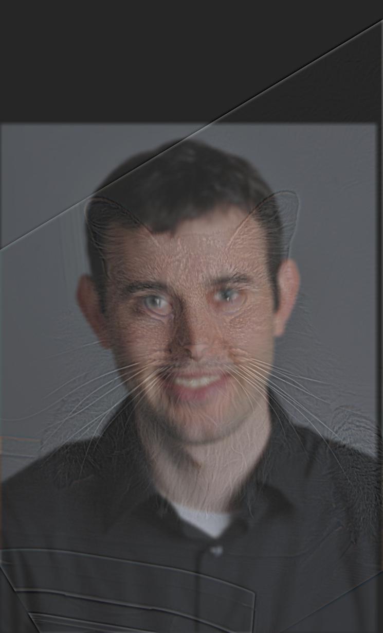
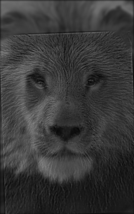
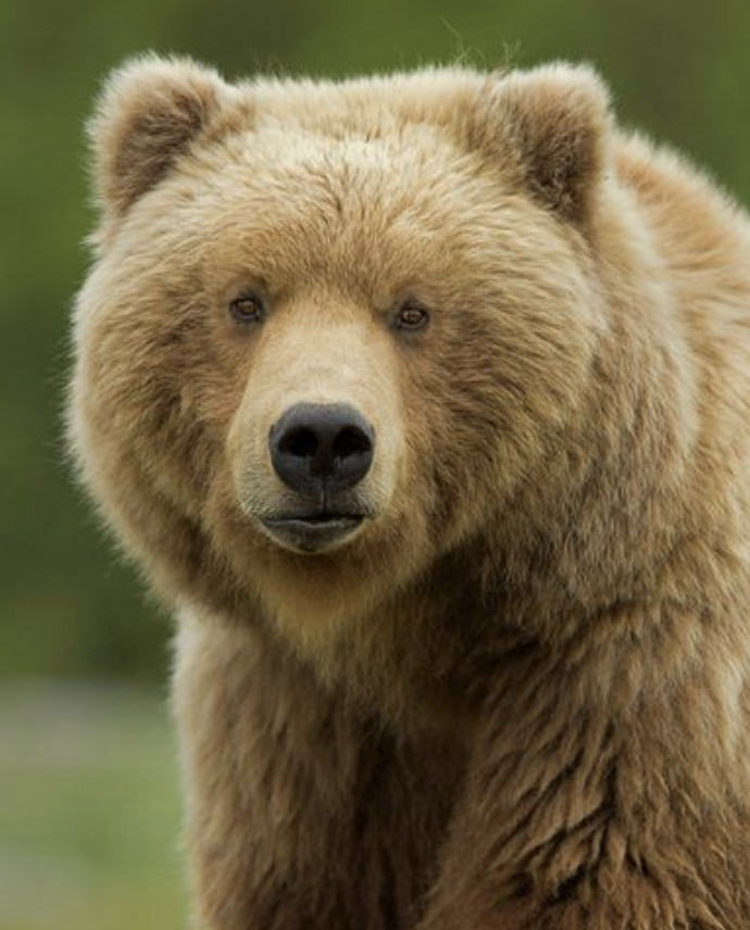
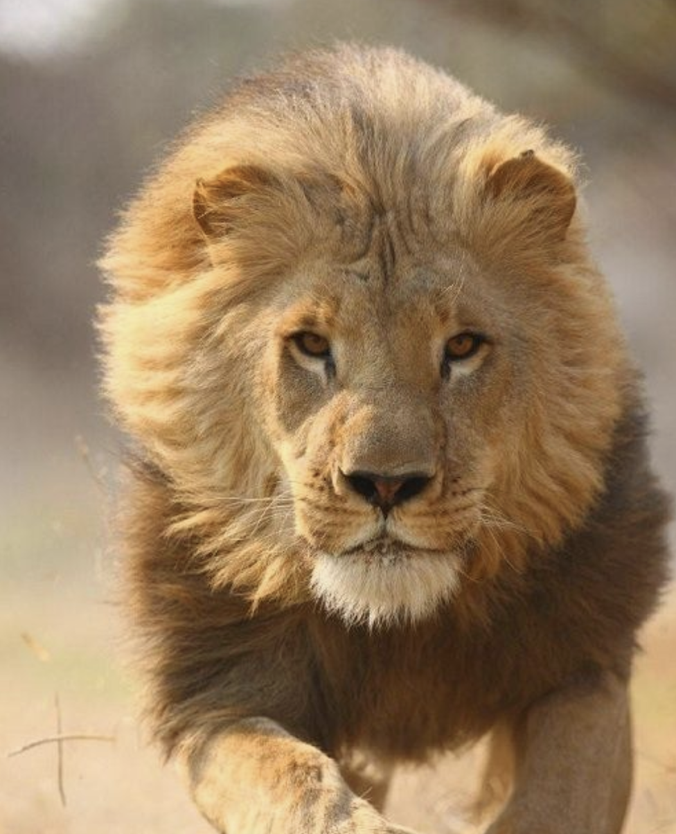
Original image with a sigma 11 blur.	Sharpened with an alpha of 0.7
Just the high frequencies for reference.

Hybrid images

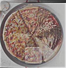
In this part, we create hybrid images by adding high frequencies from one image, to a low frequency image of another. Here are some examples of the results.

Image of Derek and his cat.	Derek	Cat
Image of a bear and a lion. This was a failure since the lion and bear both have high frequency detail and not much low frequency detail.	A bear.	A lion.

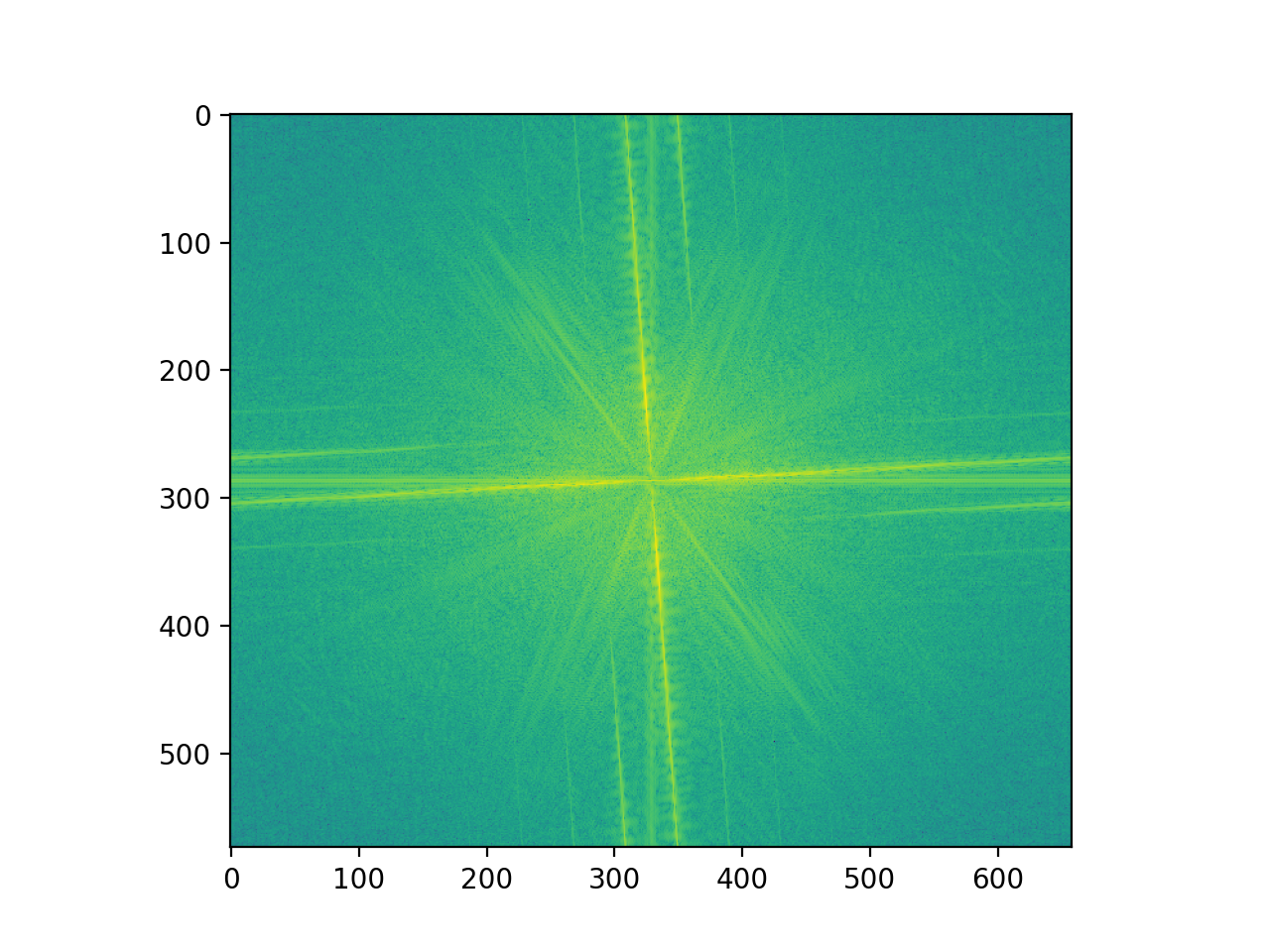
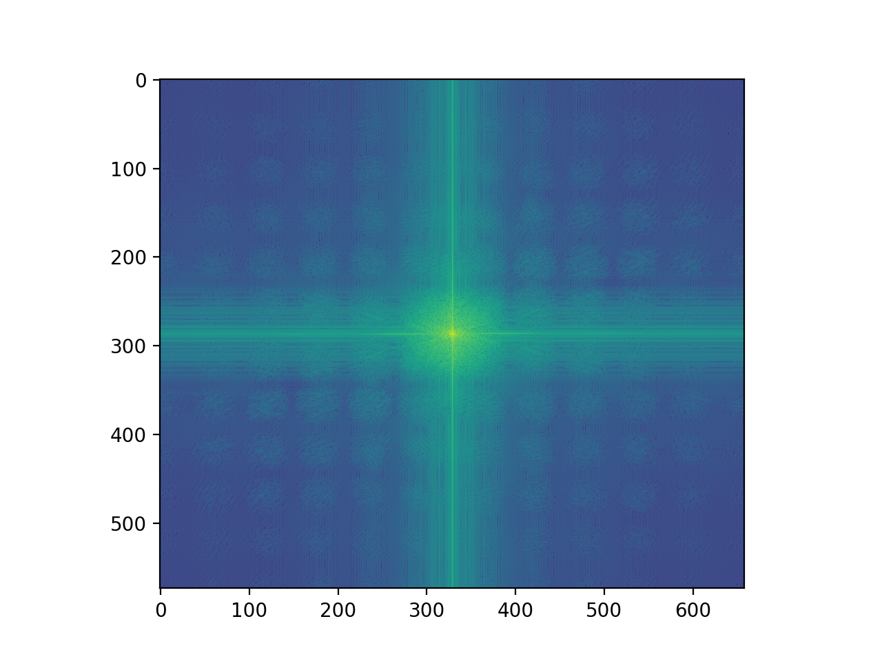
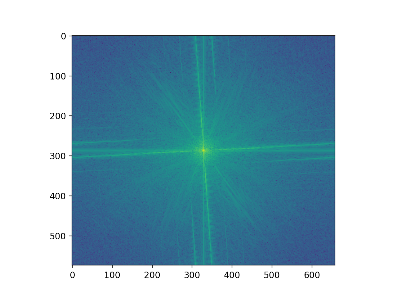
Here is a look into the process of combining these images. We show the images in the fourier domain in order to show the reduction of frequencies much clearer. We also show the laplacian and gaussian stack for these images in order to see which features of the images are being removed/contributed not in the fourier domain.

Joey after removal of low frequencies in the fourier domain	Divi after blurring in the fourier domain
Divi and Joey.	Divi and Joey in the fourier domain.
Divi's laplace and gaussian stack	Joey's laplace and gaussian stack.

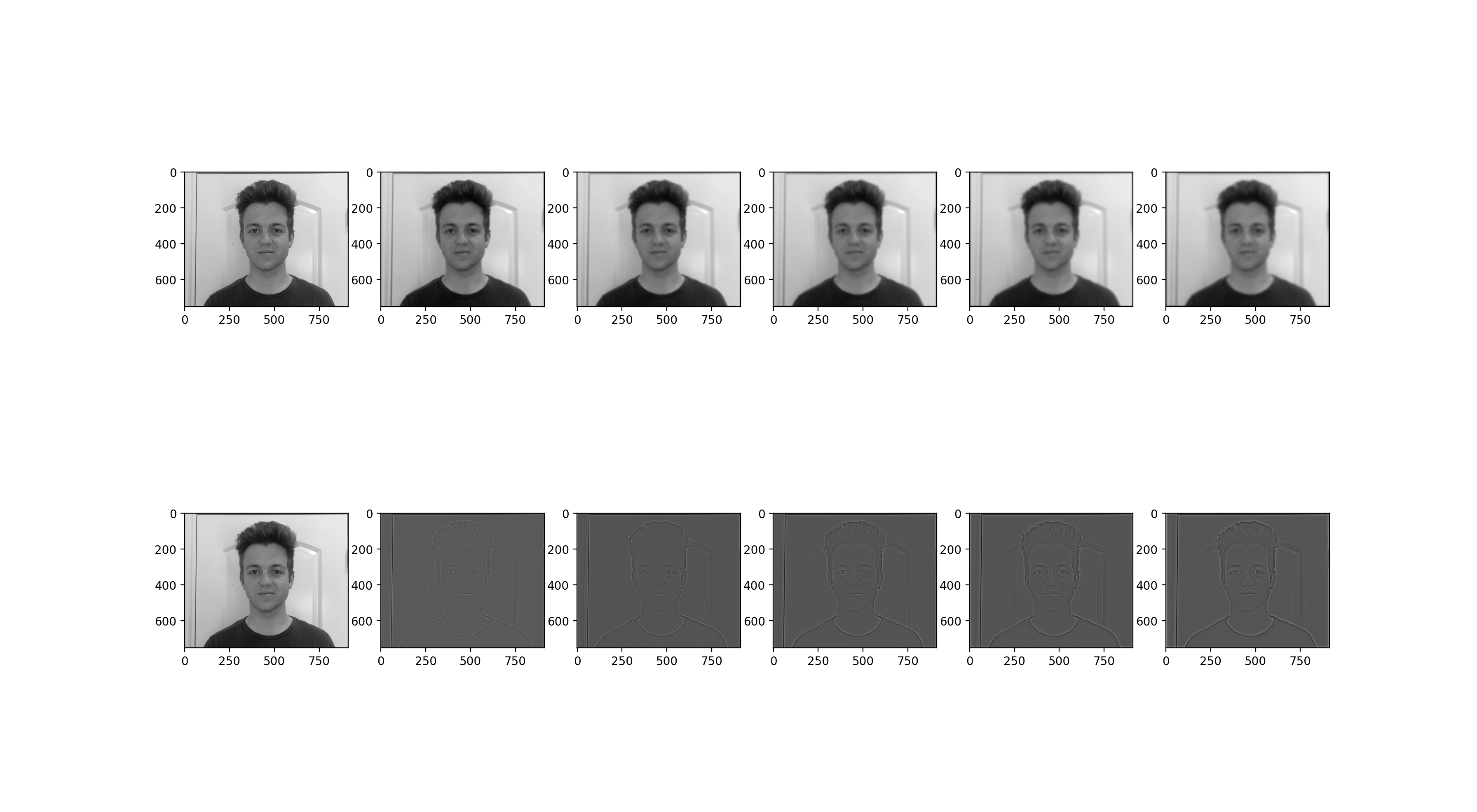
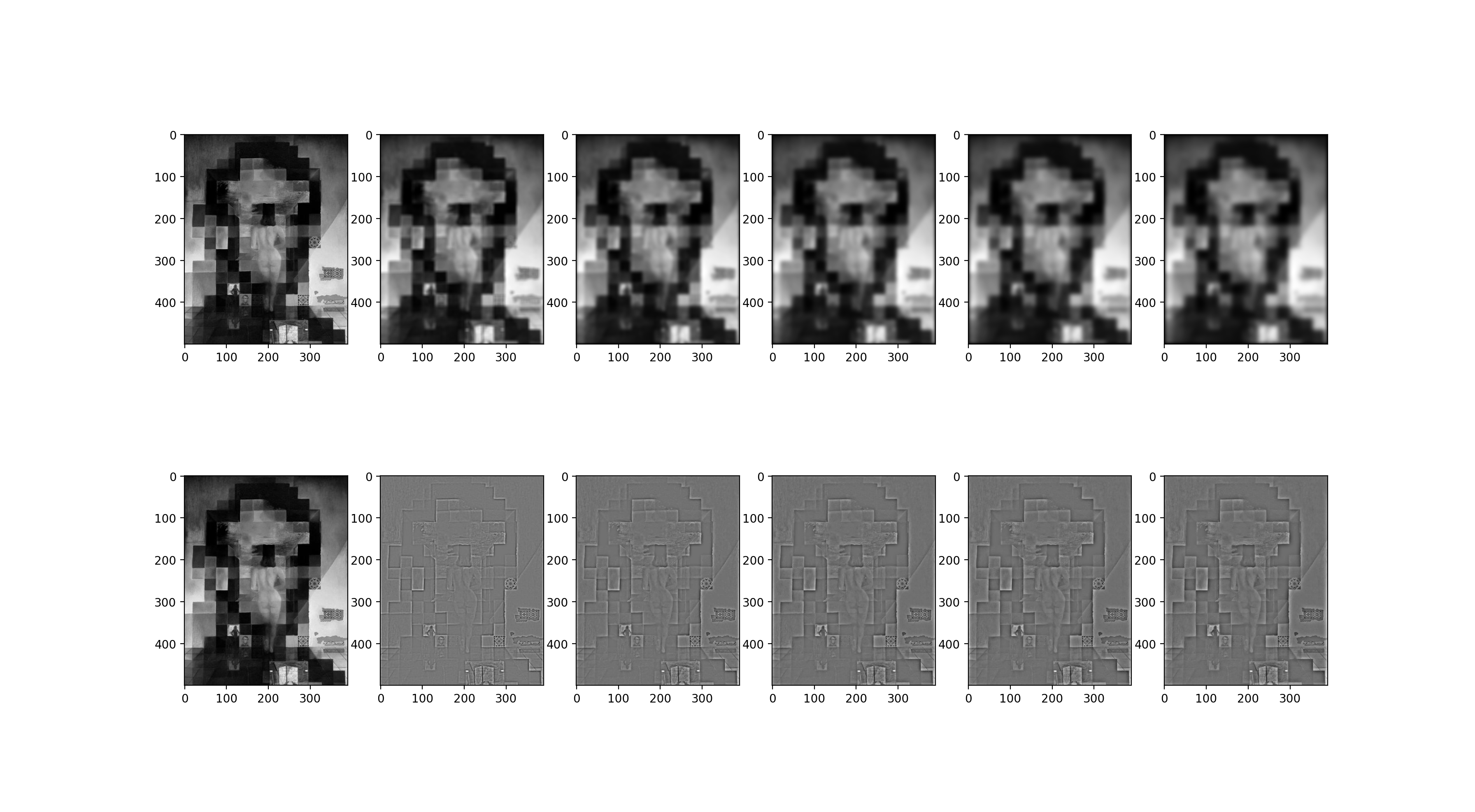
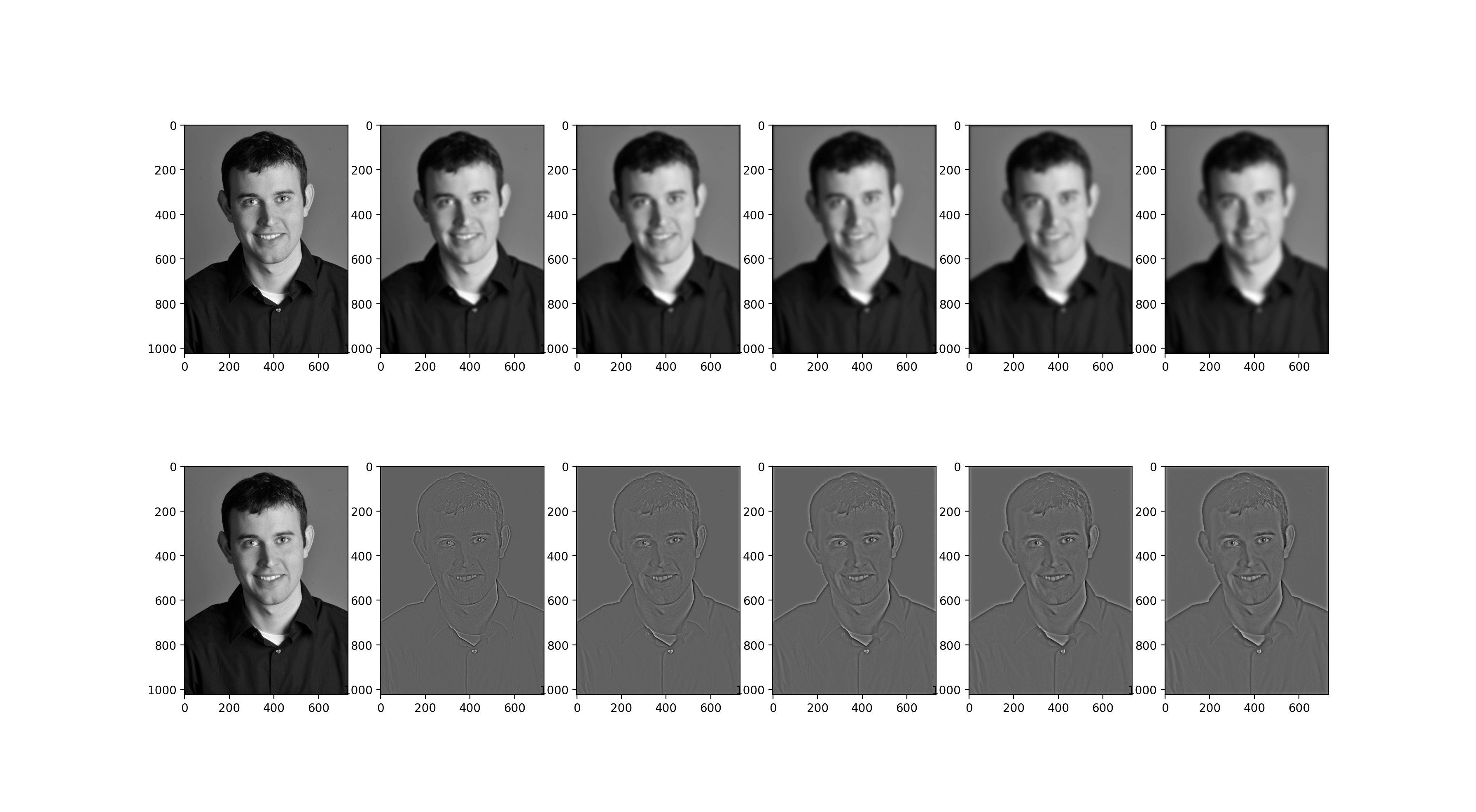
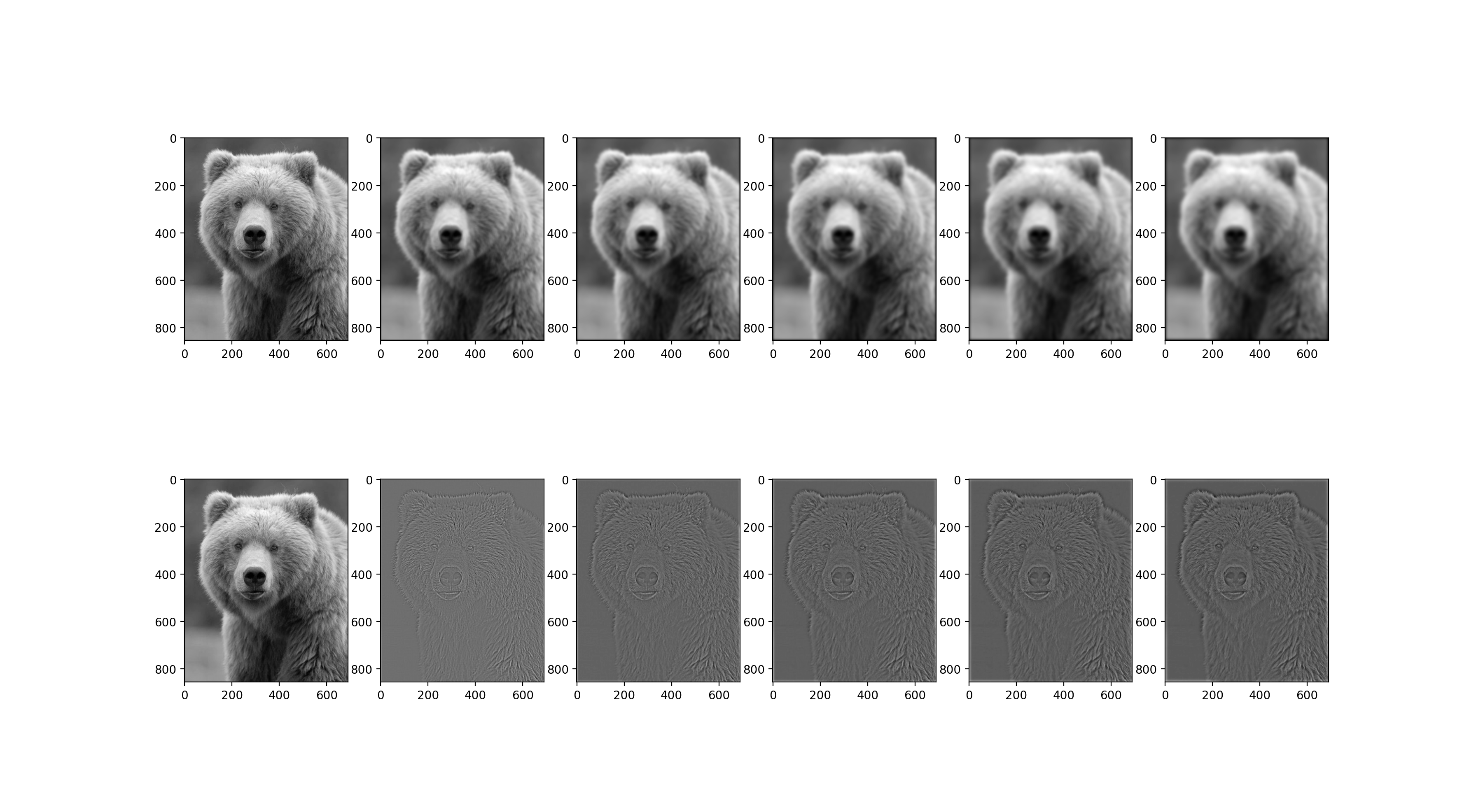
Now to gain more understanding of what these laplacian and gaussian stacks are, we show the stacks for an interesting photo with a lot of high and low frequencies. Notice how different the details are or lack of details are.

The lincoln painting	Derek
Bear.

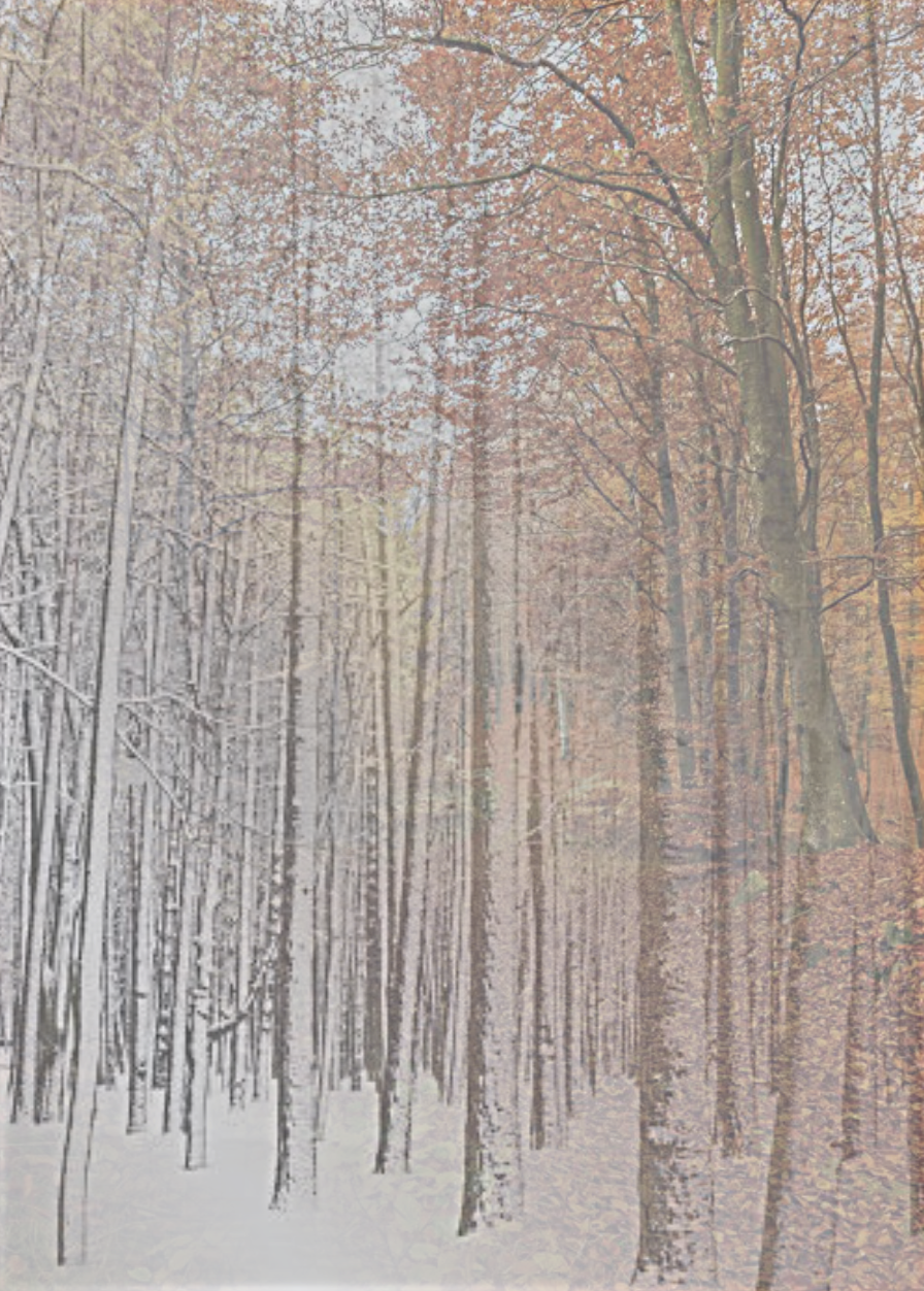
Multiresolution Blending

Here are some examples from the normal multiresolution blending technique.

the orapple	pizza and cheesecake. I thought it would look more yummy.
multiresolution blending with a different mask. The original mask was rotated and padded so that it was a diagonal blending. I think it looks better than the other method for this photo.