Project 1
Divi Schmidt
Overview
In this project, I colorized very old black and white photographs. The colors came from a combination of three images,each taken with a different color filter, and thus giving us the three rgb color channels needed for a color photo. The difficult part of this project was aligning these three images, as they were not taken from the exact same position, nor aligned perfectly when they were uploaded together. In this overview, I will walk you through the approach that i took to combine these images, and the problems I encountered along the way
The Approach
The first approach that I took was the most simple one. First, I split the image into three equal parts. Then, I performed an exhaustive search over a -15 to 15 pixel area and took the best alignment of the two channels. In order to determine the best alignment of the two channels, I implemented two different image metrics: Sum of Squared Distances and Normalized Cross Correlation. The results from these metrics are in the results section below.
Normalized cross correlation did not work very well, and sum of squared distances does
produce some good-looking results. Across the many more images, however, it is clear that some of the images
need a much more rigorous metric to determine the best alignment.
Additionally, this implementation was very slow on the larger tif files, which sometimes also require larger
search windows. In order to solve this problem. I implemented search with an image pyramid. This meant that
I first searched a small window using a very scaled down image (1/16 or 1/32, I didn't notice a big
difference between the two). Then, when I moved one step down in the image pyramid, I searched a small area
around the previously determined best alignment. This allowed for a very large speedup, making the
conversion for most large images take ~7 seconds to complete.
Thoughts on Failure
Thoughts
If your algorithm failed to align any image, provide a brief explanation of why.
The original problem that I encountered with aligning images was buggy code. Without much of a way to test, I struggled to figure out if my alignmnet was a result of a bug in my code, or just because my metrics were not good enough to properly align images. After a lot of frustration, I finally did the wise thing and created a test image that I knew the exact offsets for and could therefore test my code with.
Although there are some very promising results as shown above, there are also some images that fail with the same metrics. The reason for this can vary with each image so I will talk about a couple specific cases.
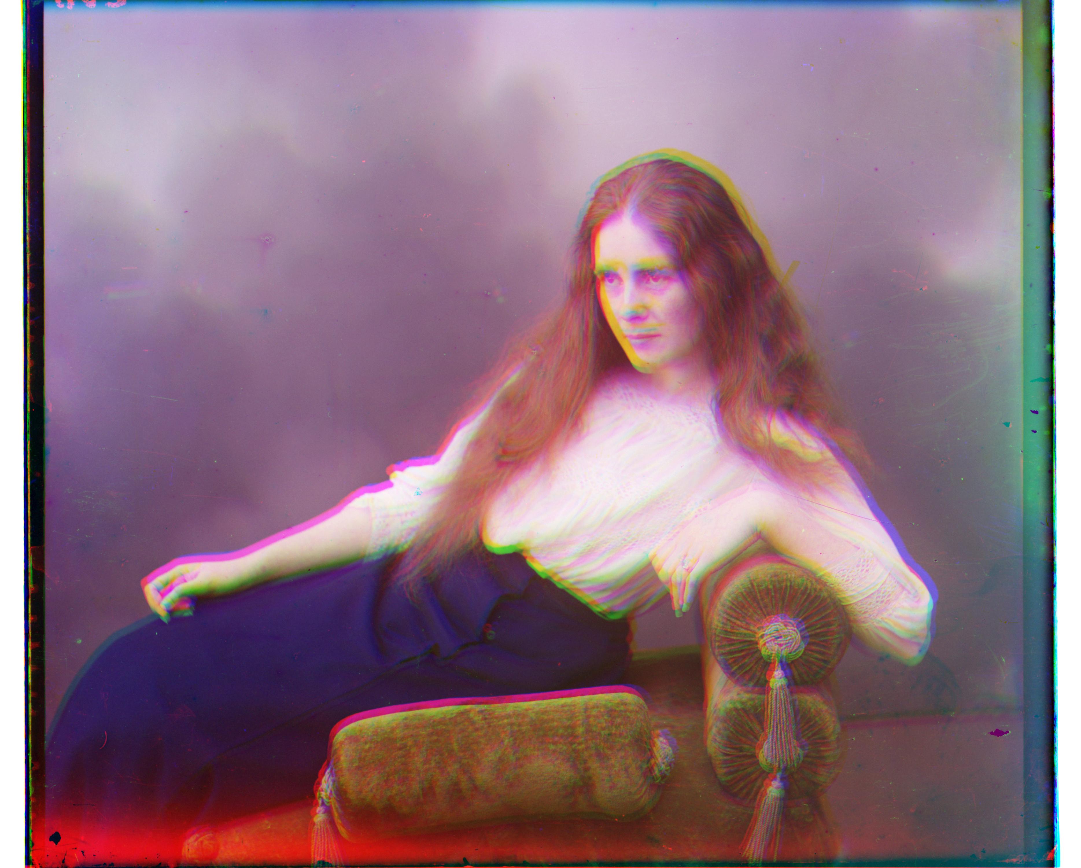
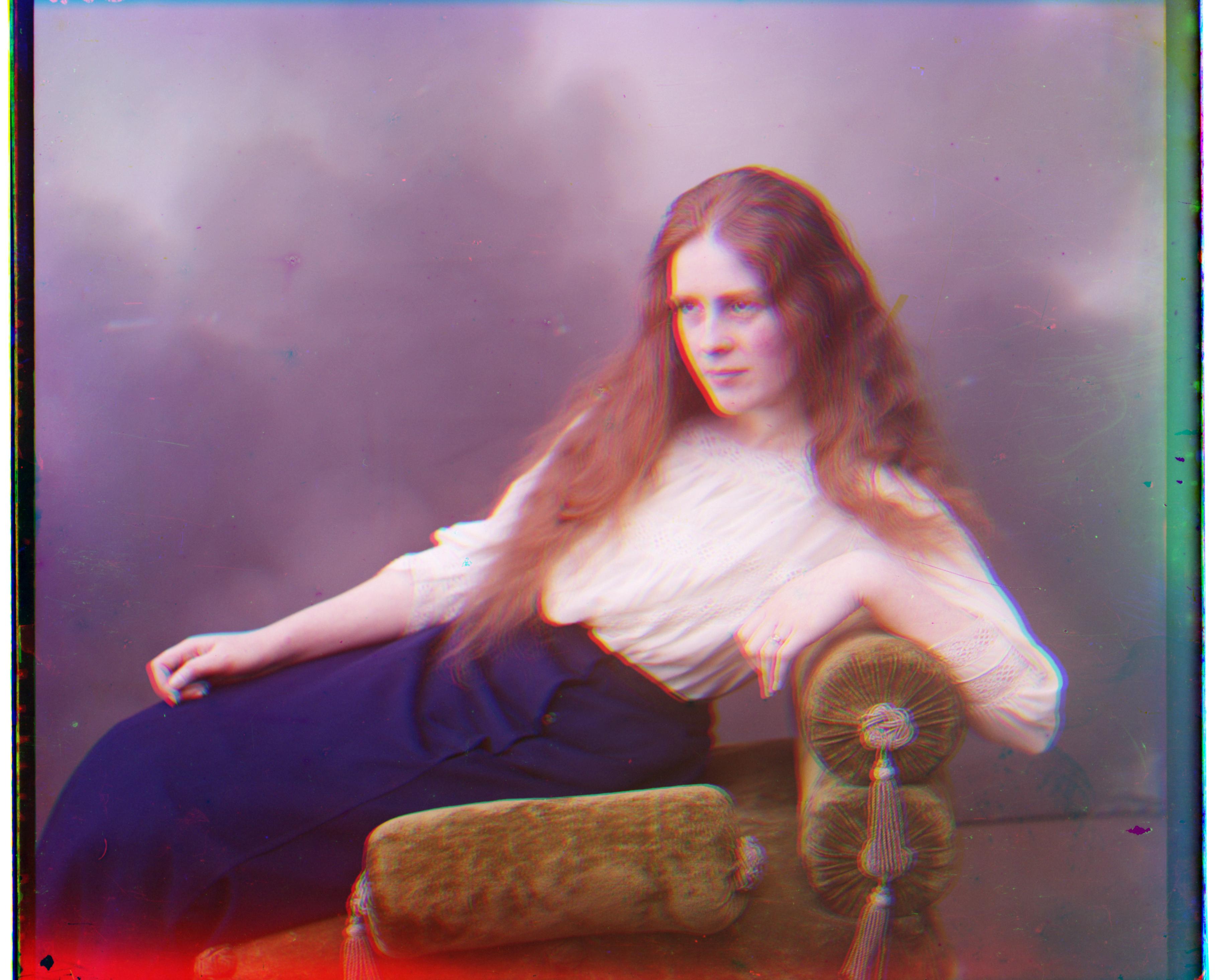
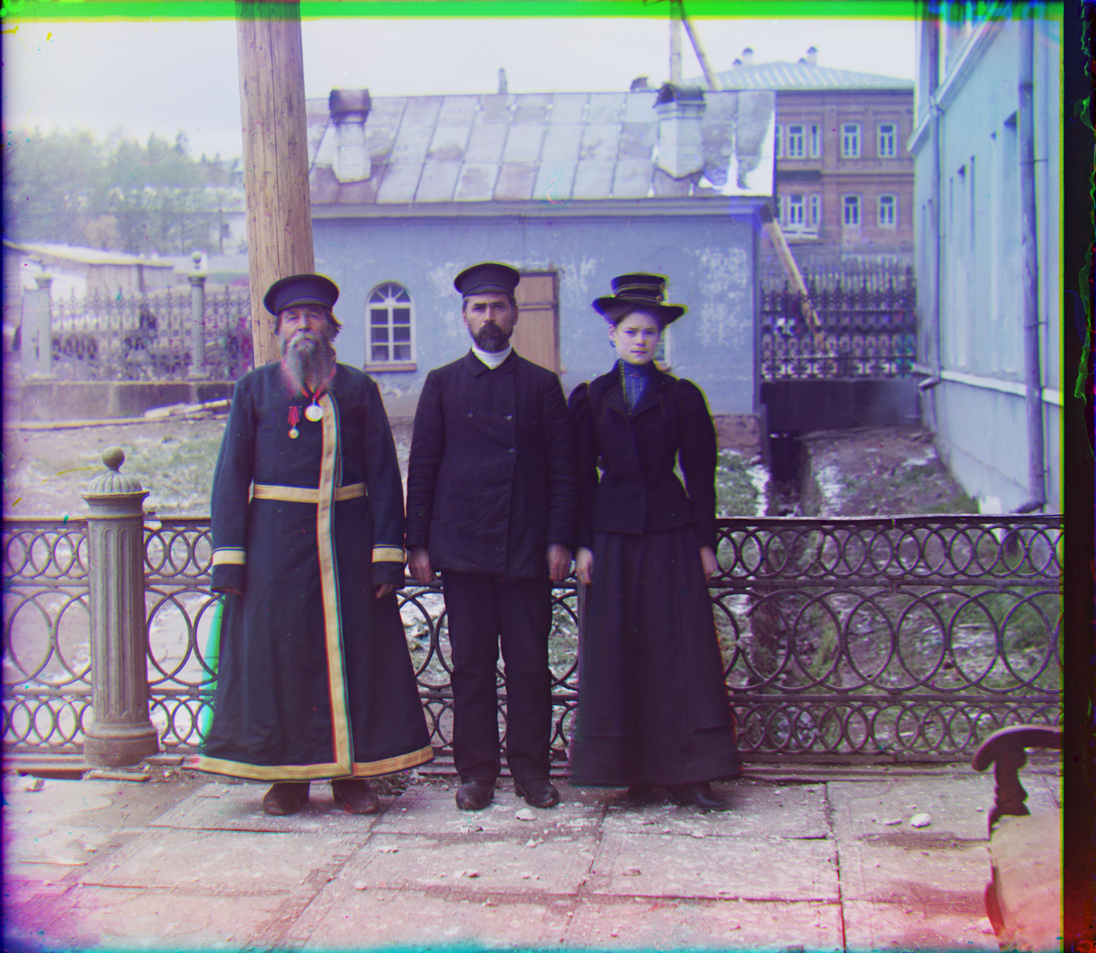
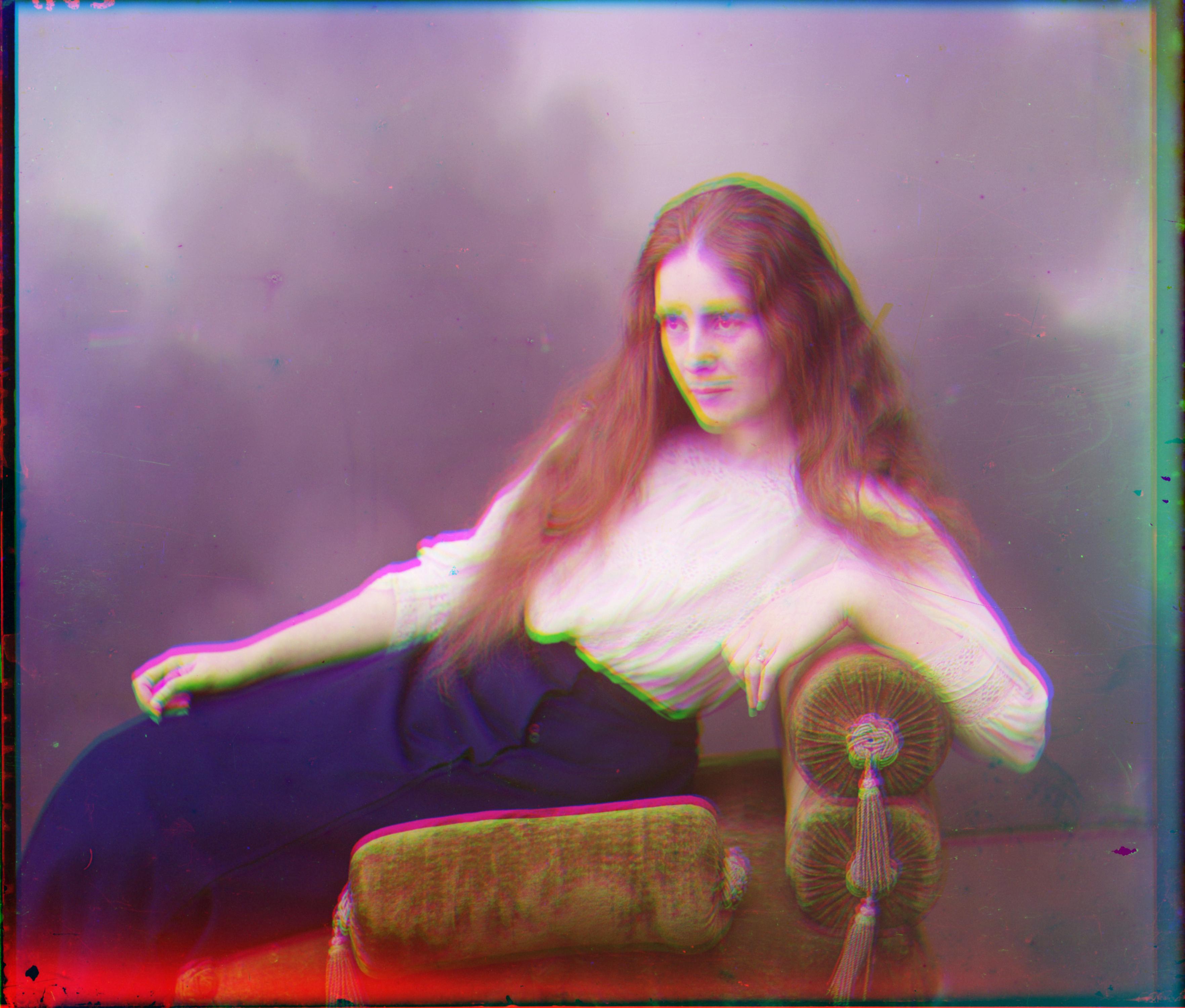
For this image, I believe that the streaks on the bottom of the image throw off my alignment algorithm. The red streak is quite large and distinct, which causes the ssd to have a high error if this streak is not aligned. Clearly, we do not care if it is aligned, but we are not the ones determining the offsets. To test out this theory, I cropped the lady image by 50 pixels on each side for each channel and then ran this again. As you can see, this improved the alignment a lot and the red light streak is much smaller.
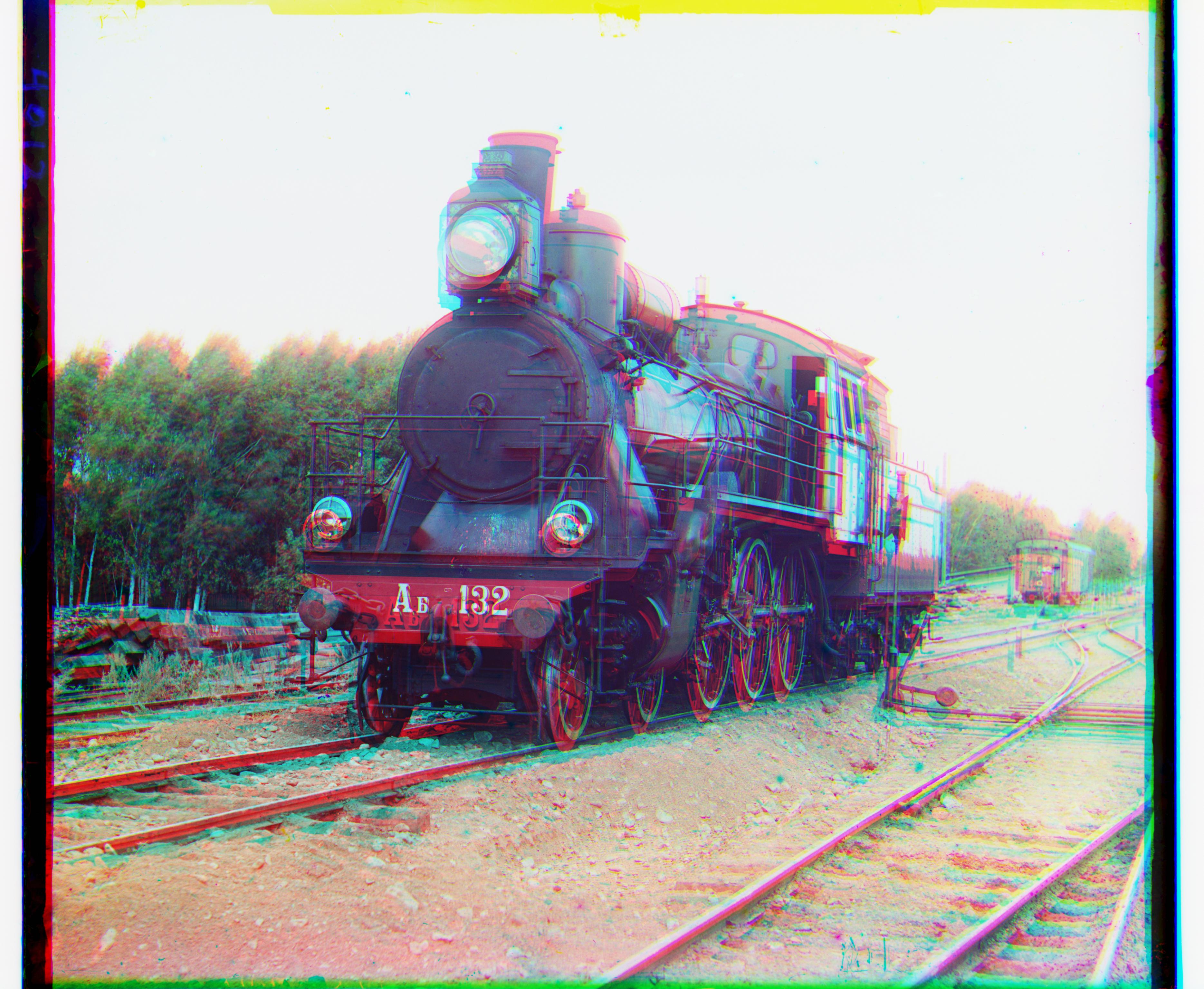
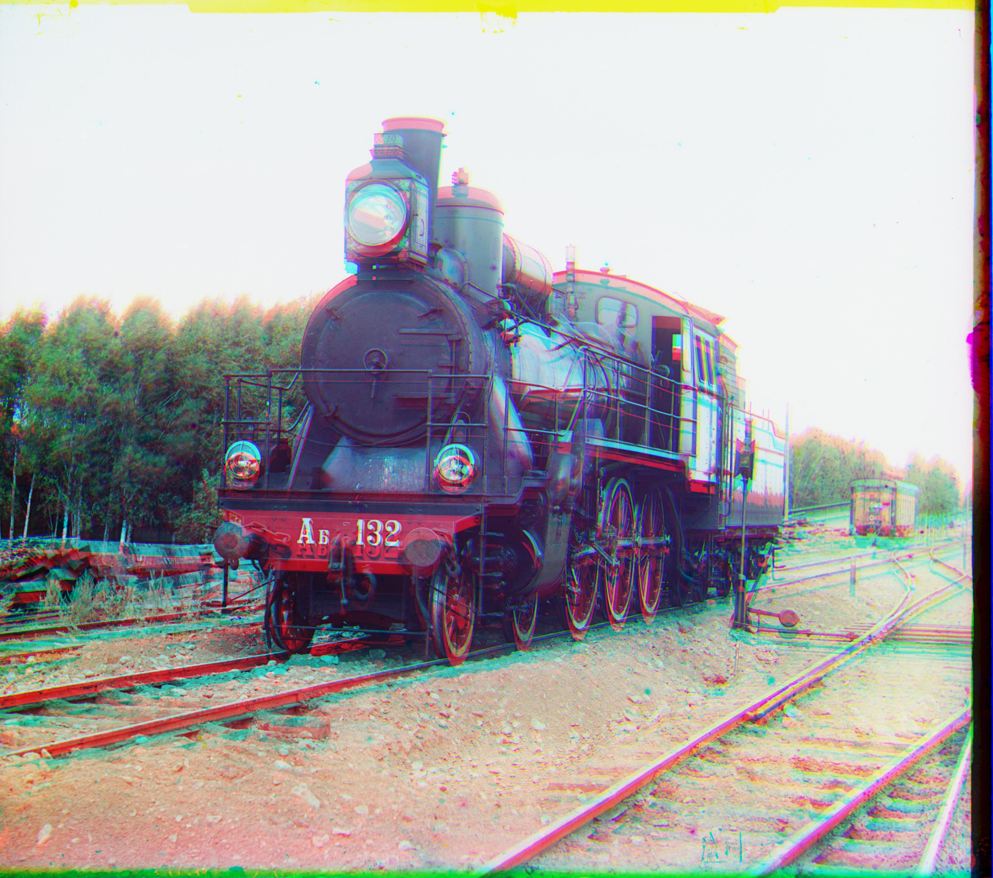
For the other images that failed, I observed that they had the same strange borders or image degradations that we saw with the lady. Here is another example. The top channel has a very dark border that is throwing off the alignment of the train.
Bells and Whistles
These were an attempt at solving the issues we saw above.
Weighting SSD
My first attempt at fixing this was to naively weight the pixels in the image so that the SSD would return a higher error when the center was not aligned, instead of biasing towards the borders. I did this by creating an array that had very large values in the center of the image, and low ones around the borders. This did not work well as it was operating under the assumption that the center was always the most important part of the image.
My second attempt at fixing this was to weight the pixels using the canny edge detector. This caused the edges in the image to be weighted much higher than the other parts of the image. This did not directly solve the border problem, however it did weight the important parts of the image since there were borders detected around people and other important objects.
Automatic Border Cropping
Instead of trying to improve the image metrics further, I instead opted to implement automatic border cropping in an attempt to clean up the images and hopefully get better aligned images. I tried two different methods for this.
Canny Edge Detection
My first attempt was using canny edge detection. However, I found it difficult to determine the best way to use the information gleaned from this edge detector. The detector outputs an array the same size as the image, but with boolean values for each pixel: edge or no edge. This array was very noisy as it was not clear what was a border aka what we wanted to crop, or just an edge in the image aka very useful information. In order to circumvent this, I only searched over the first 1/8th or last 1/8 of the image when looking for the border of the image. Now in this window, I then took the column with the maximum number of edge detections, and cropped the image on this column. This did not give good results and the crops often cropped off important parts of the image instead of the borders. This is the reason why I tried to use this for the pixel weighting as described above, as it seemed much more useful in this case.
Horizontal Gradient
In order to determine where the actual borders of the image were, I instead simplified my edge detection algorithmm by taking the gradient only along the horizontal. This meant taking the value of Image[j, k + 1] - Image[j, k - 1] for each pixel. This was very successful in detecting only the left and right borders of the image, and nothing else. Here is an example:
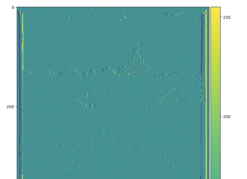
In order to detemine where the edges were. I then counted all gradients above 150 as an edge, and everything else as not an edge. Then I took the sum for each column and took the argmax for the left half and the argmax for the right half. Here is a plot of the column sums as as reference for the utility of this method.
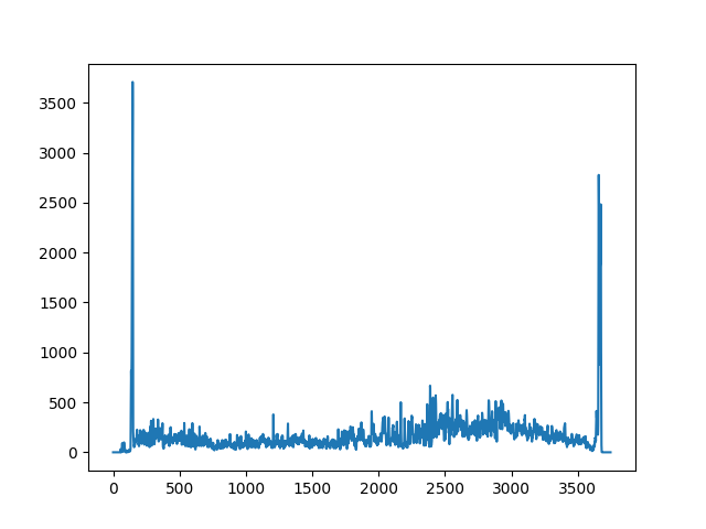
As you can see, it is very clear where the left and right border is, and these calculations are not distracted by the other non vertical edges in the scene. All of the images in the results section are using this edge removal algorithm, but here are before and after images to see the real affect of this method.
|
|
Vertical Gradient
The last thing that I tried was to detect the horizontal borders and determine a better way to split the image in to three separate channels. However, this did not work at all. The edges that were detected were in the center of the image and rarely on the horizontal line. Looking at some more images, these separation points are not very distinct a lot of the time. Some of these borders are just light grey, which made it very difficult to detect with the canny edge detection or by taking a vertical gradient of the image. So I reverted back to the original separation method.
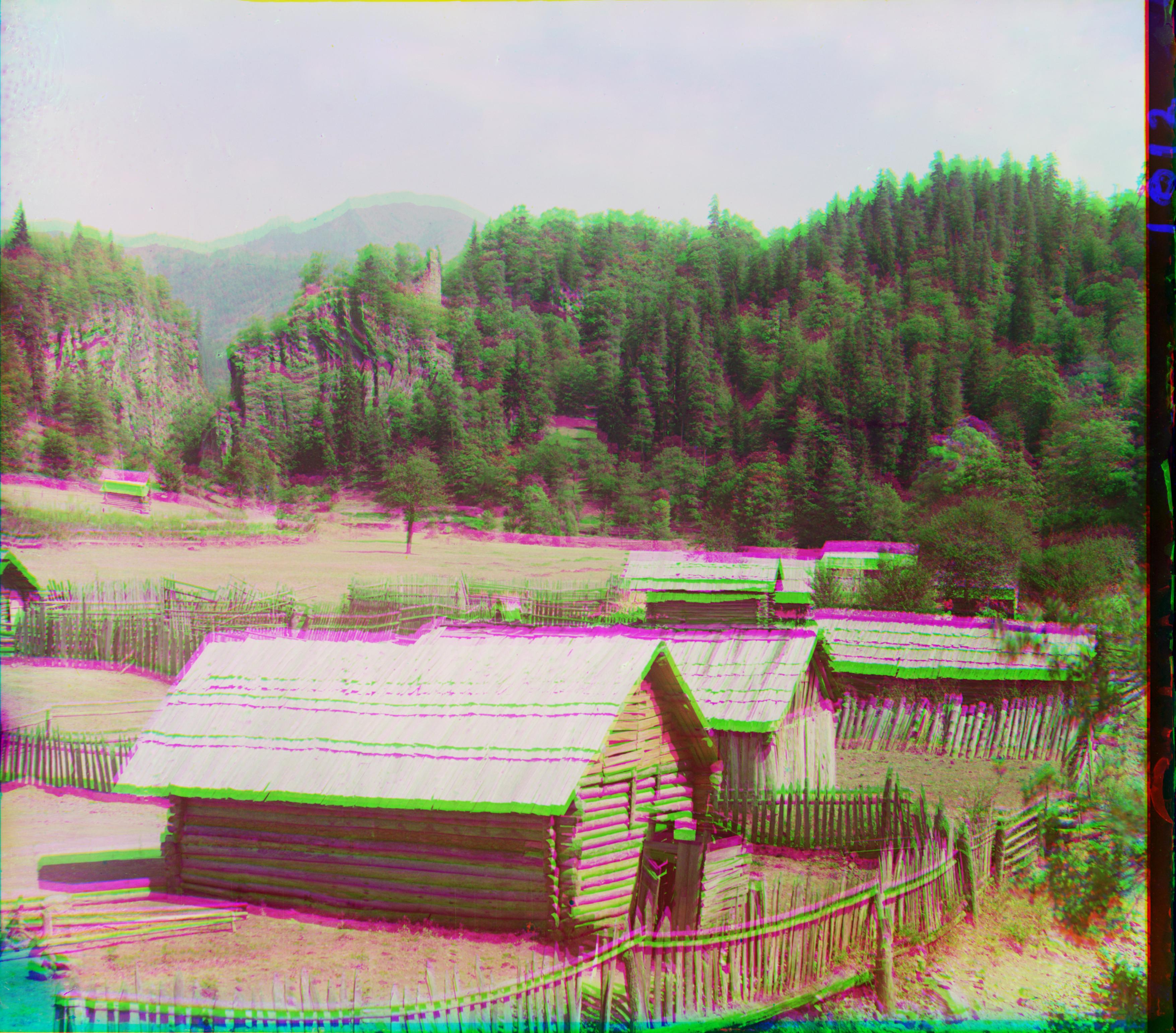
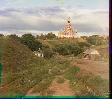
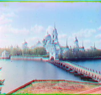
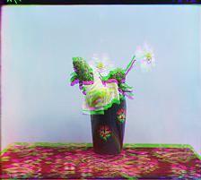
Results
All Example Images
|
|
|
|
|
|
|
|
|
|
|
|
|
|
|
Offsets
Converting workshop.tif
Removed borders of size: (90, 94)
Displacement for G channel: (-54, 2)
Displacement for R channel: (-101, 13)
Time elapsed: 15.157158136367798
Converting emir.tif
Removed borders of size: (95, 82)
Displacement for G channel: (-49, -24)
Displacement for R channel: (-106, -42)
Time elapsed: 15.426254034042358
Converting three_generations.tif
Removed borders of size: (98, 92)
Displacement for G channel: (-54, -12)
Displacement for R channel: (-114, -10)
Time elapsed: 14.984628915786743
Converting castle.tif
Removed borders of size: (69, 89)
Displacement for G channel: (-66, 2)
Displacement for R channel: (-98, -3)
Time elapsed: 15.638453006744385
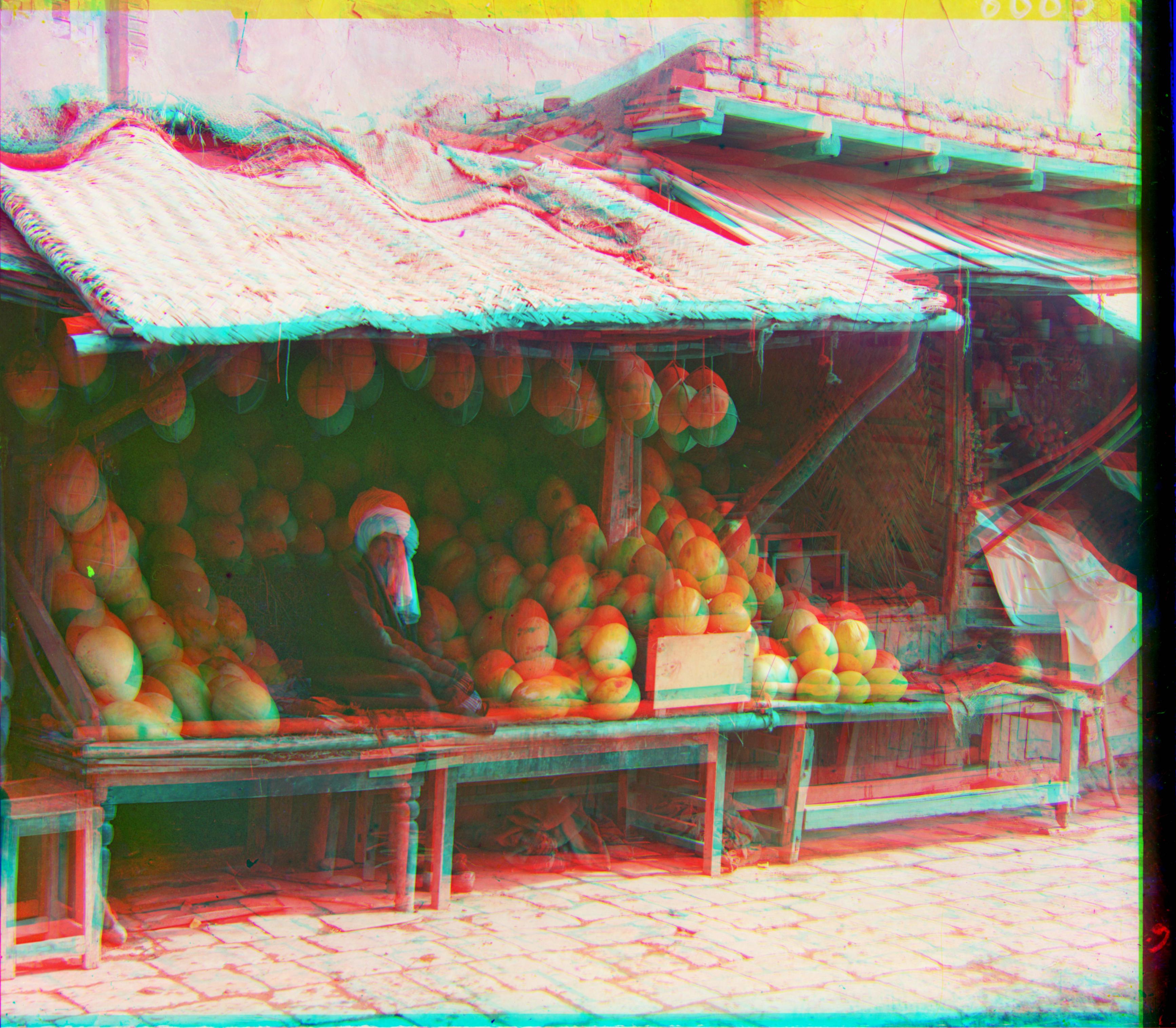
Converting melons.tif
Removed borders of size: (98, 96)
Displacement for G channel: (-83, -4)
Displacement for R channel: (-126, 17)
Time elapsed: 15.753090143203735
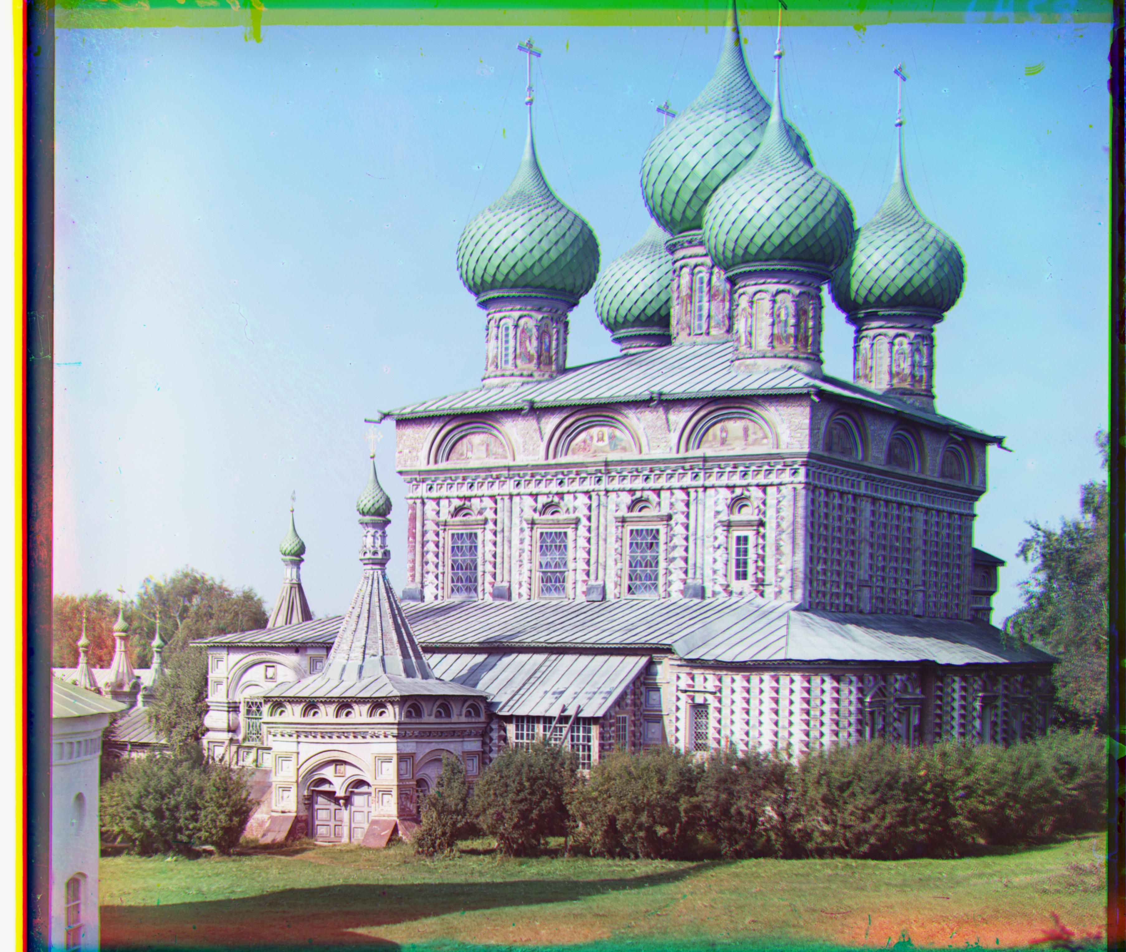
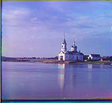
Converting onion_church.tif
Removed borders of size: (0, 100)
Displacement for G channel: (-53, -23)
Displacement for R channel: (-108, -36)
Time elapsed: 16.50060486793518
Converting train.tif
Removed borders of size: (68, 86)
Displacement for G channel: (-42, 2)
Displacement for R channel: (-126, -15)
Time elapsed: 16.243185997009277
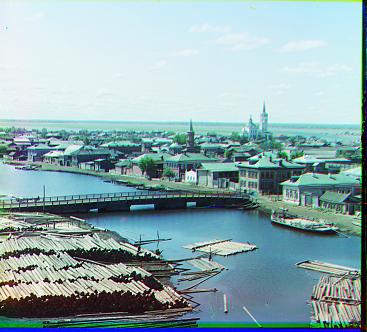
Converting tobolsk.jpg
Removed borders of size: (16, 7)
Displacement for G channel: (-3, -2)
Displacement for R channel: (-6, -3)
Time elapsed: 0.16897296905517578
Converting icon.tif
Removed borders of size: (91, 89)
Displacement for G channel: (-42, -17)
Displacement for R channel: (-91, -23)
Time elapsed: 1.064661979675293
Converting self_portrait.tif
Removed borders of size: (0, 100)
Displacement for G channel: (-76, 1)
Displacement for R channel: (-126, 5)
Time elapsed: 16.578269004821777
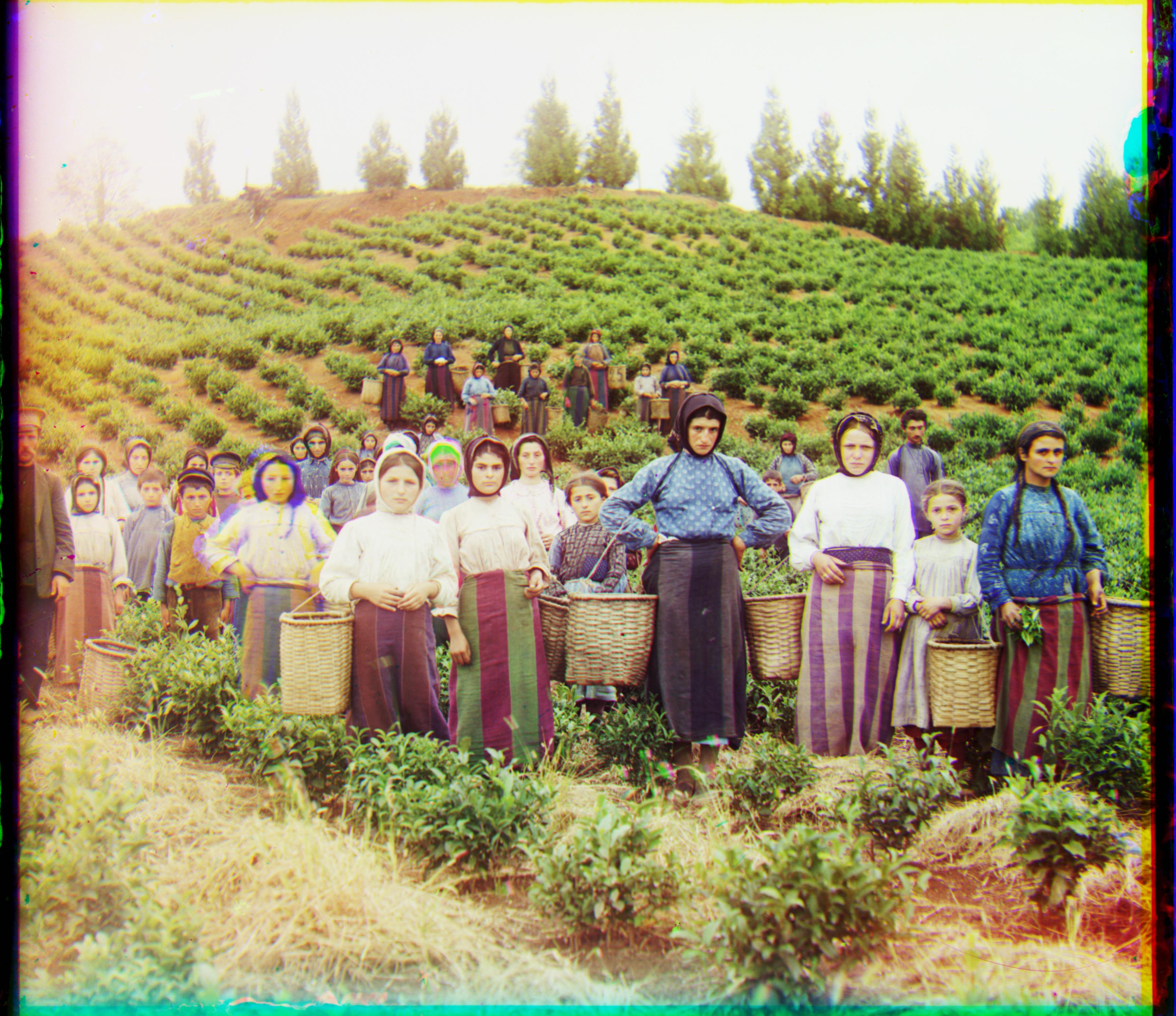
Converting harvesters.tif
Removed borders of size: (64, 83)
Displacement for G channel: (-60, -15)
Displacement for R channel: (-126, -13)
Time elapsed: 15.875388860702515
Converting lady.tif
Removed borders of size: (98, 99)
Displacement for G channel: (-87, 8)
Displacement for R channel: (-125, 12)
Time elapsed: 16.103732109069824
Converting monastery.jpg
Removed borders of size: (17, 14)
Displacement for G channel: (3, -2)
Displacement for R channel: (-7, -3)
Time elapsed: 0.45801305770874023
Converting tobolsk.jpg
Removed borders of size: (17, 8)
Displacement for G channel: (-3, -2)
Displacement for R channel: (-6, -3)
Time elapsed: 0.444627046585083
Converting cathedral.jpg
Removed borders of size: (12, 8)
Displacement for G channel: (-5, -2)
Displacement for R channel: (-12, -3)
Time elapsed: 0.4329562187194824
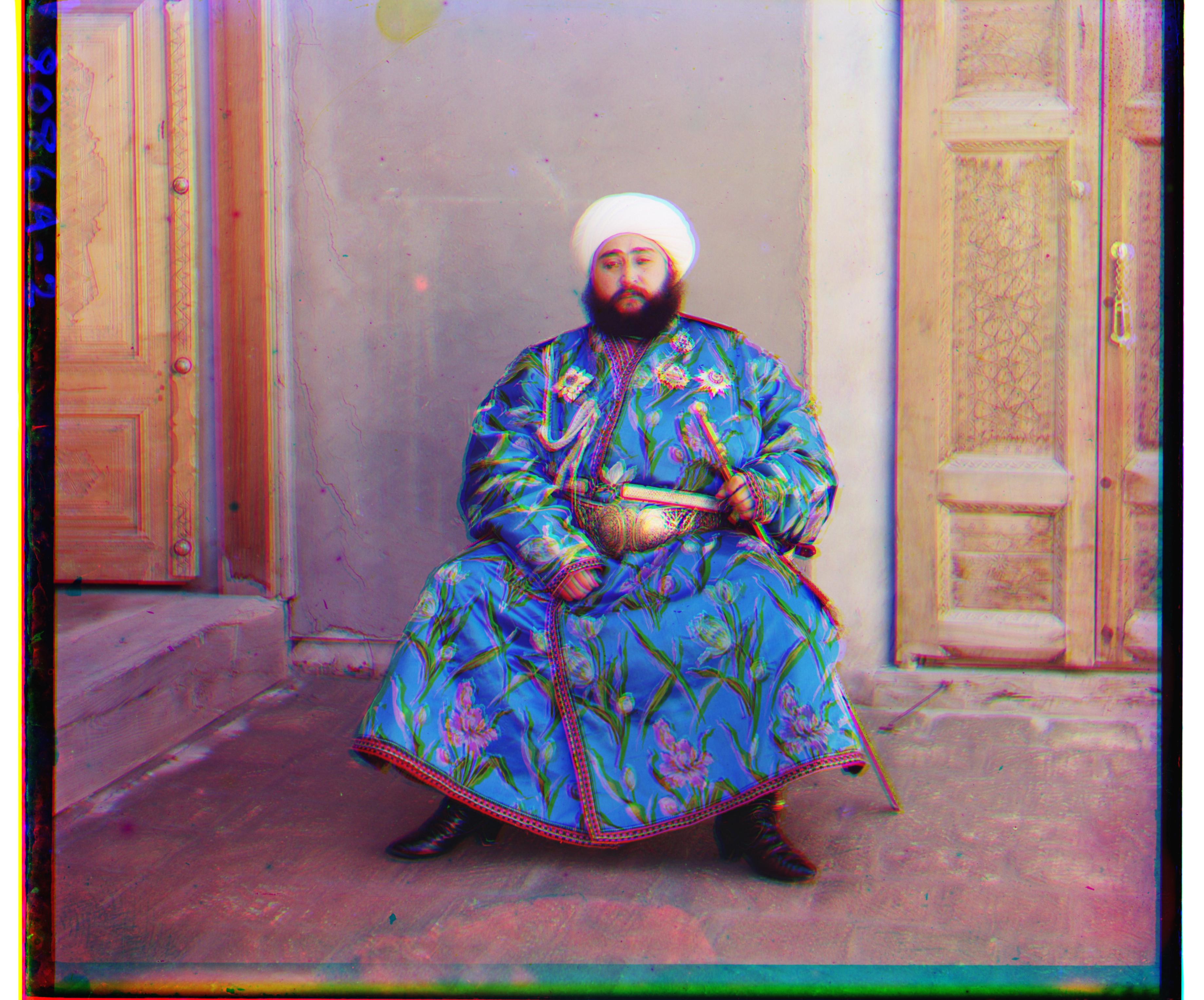
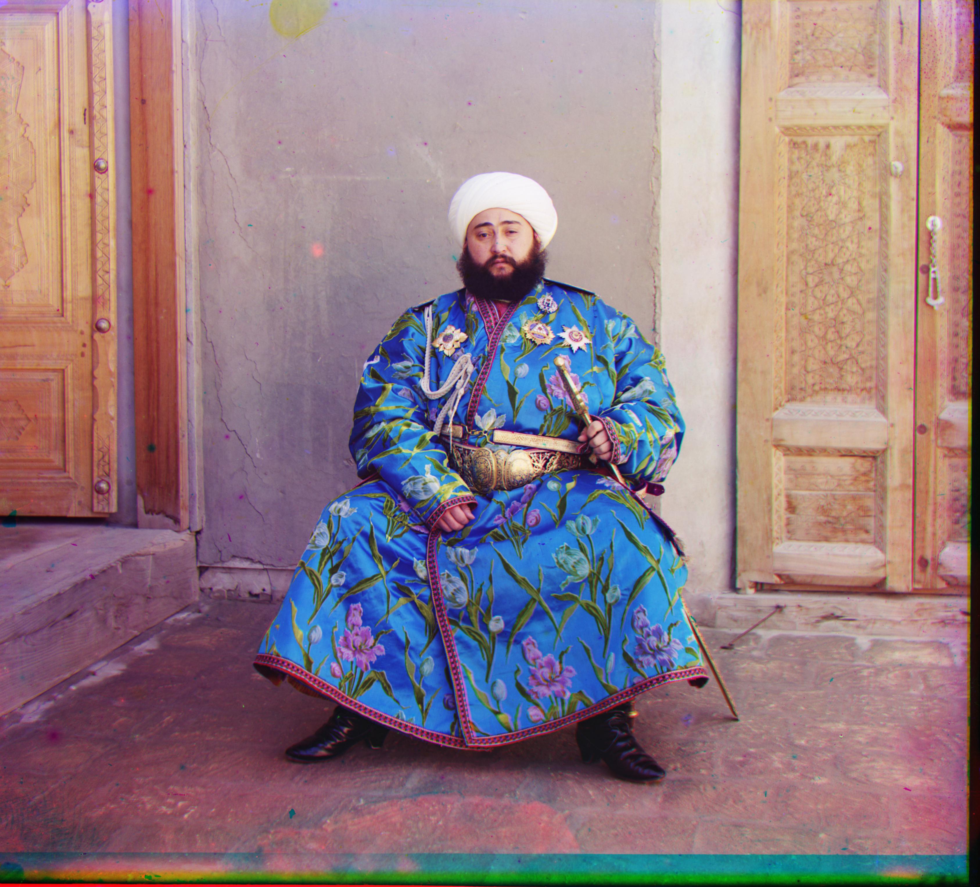
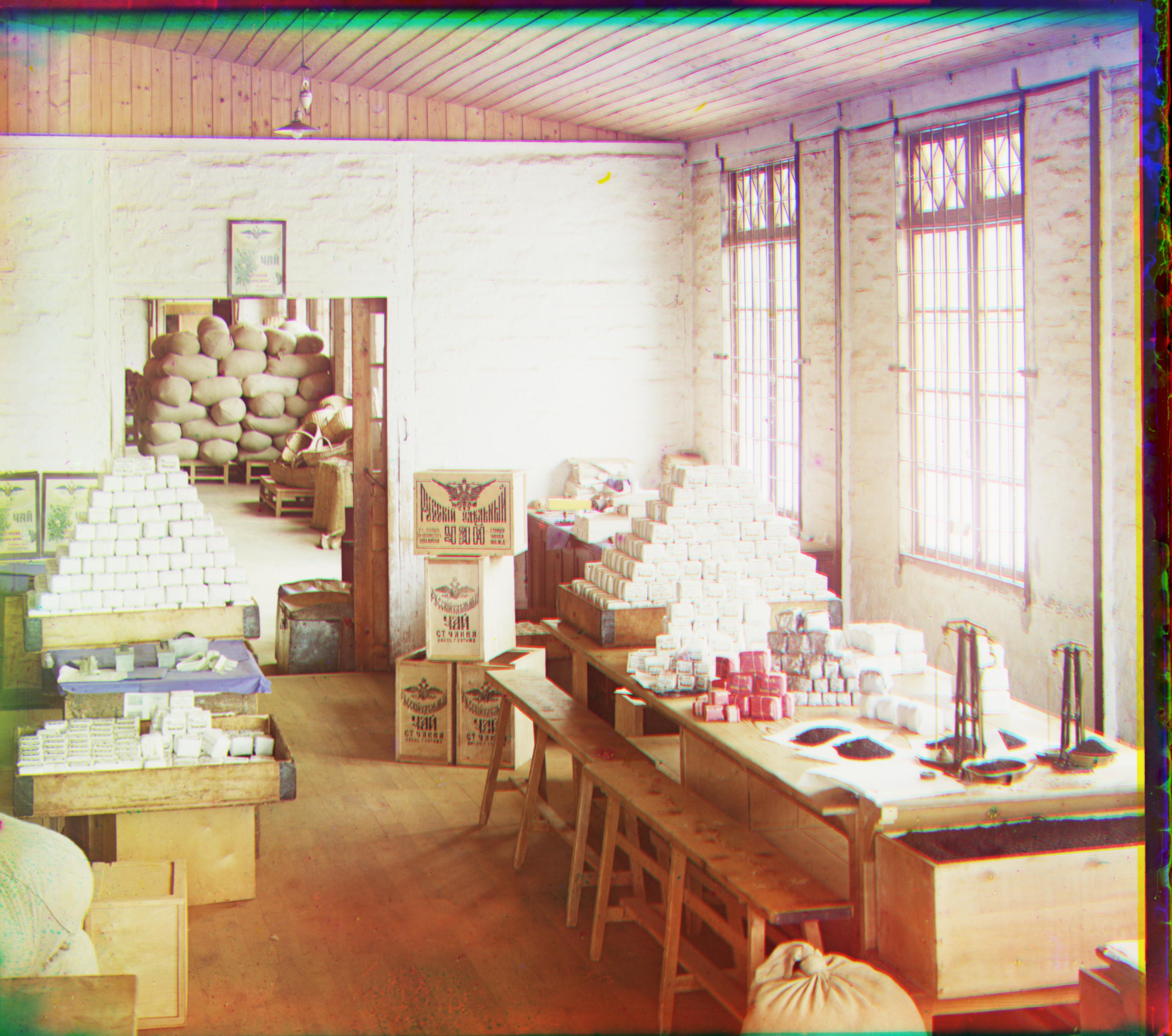
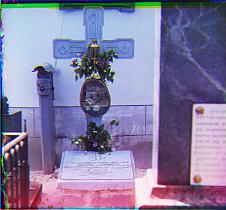
My Chosen Images
The result of your algorithm on a few examples of your own choosing, downloaded from the Prokudin-Gorskii collection.
|
|
|